Chapter 4: Vibrational Motion#
Prof. Eugene DePrince, Florida State University, and Prof. Jay Foley, UNC Charlotte
In the previous notebook, we discussed quantum mechanical problems involving translational motion: the free-particle, the particle-in-a-box model, the finite square well potential model, and tunneling through a one-dimensional potential energy barrier. In this notebook, we continue exploring model problems, with a focus, this time, on vibrational motion. In particular, we will find analytic solutions the Schrödinger equation for the (one-dimensional) quantum harmonic oscillator model, which captures the main qualitative features of vibrational motion in molecular systems.
The Harmonic Potential#
A harmonic oscillator is a system that, when displaced from its equilibrium position, experiences a harmonic restoring force, which is proportional to the displacement. In one dimension, this force would be
where \(x - x_e\) is the displacement from the equilibrium position, \(x_e\), and \(k\) is the proportionality constant, which is called the force constant. Recall that force and potential are related by
Integrating this expression yields the potential
where \(c\) is an arbitrary additive constant. This constant will not affect the solutions to the classical or quantum harmonic oscillator problems, but it will provide an arbitrary shift to the associated energies. For convenience, we choose \(c = 0\), and we proceed with the potential
Because the harmonic oscillator problem is a model for molecular vibrations, it will be illustrative to consider how this potential relates to one for an actual molecular system. We will consider the diatomic carbon monoxide, CO. Below, we will calculate the potential energy curve along the bond stretch coordinate for CO using a procedures for finding approximate solutions to the electronic part of the Schrödinger equation, called Hartree-Fock theory. You can read more about Hartree-Fock theory in this notebook. We will use this approach in the PySCF electronic structure package, with the cc-pVDZ basis set.
The first code block will install the relevant packages for all of the PySCF calculations performed in this notebook if needed.
If you are running on Google Colab, you should run these every time you run this notebook
If you are running locally, you can run these commands locally only once and then you will have them for all future sessions.
!pip install pyscf
!pip install geometric
!pip install pyberny
!pip install pyscf
!pip install geometric
!pip install pyberny
The next block imports the relevant libraries from PySCF
import numpy as np
from pyscf import gto, scf # Import necessary modules
# conversion from Angstroms to atomic units
ang_to_au = 1.88973

# set molecule
mol_template = """
C 0 0 0
O {} 0 0
"""

hf_potential = []


dx = 0.01
dx_au = dx * ang_to_au

# array of bond lengths in angstroms, which will be what PySCF understands
x = np.arange(0.5, 2.05, dx)

# array of bond lengths in atomic units (Bohr), which is what we will use for calculating k in atomic units
x_au = x * ang_to_au

for i in range(len(x)):
    current_x = x[i]

    # Redefine the molecule for each geometry
    mol = gto.M(
        atom=mol_template.format(current_x),
        basis='cc-pvdz',
        verbose=0,
        spin=0) # Keep output quiet for each step

    # Perform RHF calculation
    mf = scf.RHF(mol)
    mf.kernel()

    # Extract the RHF energy
    hf_en = mf.e_tot
    hf_potential.append(hf_en)


# Now, all three lists will contain the respective energies for each geometry.
print("RHF Potential Energy Curve (first 5 points):", hf_potential[:5])
Now, let us visualize this potential (shifted so that the minimum value is zero)
# import matplotlib
import matplotlib.pyplot as plt

# minimum energy
V_e = min(hf_potential)


# shift potential so the minimum value is zero
hf_potential = np.array(hf_potential) - V_e


plt.figure()
plt.plot(x , hf_potential, label='Hartree-Fock')
plt.xlim(0.6, 2.0)
plt.ylim(0, 1)
plt.ylabel('potential')
plt.xlabel('C-O distance (Angstroms)')
plt.legend()
plt.show()
Near the equilibrium C-O distance, the potential in which the nuclei live looks harmonic, i.e., it could be approximated by a quadratic function. How can we extract an appropriate force constant, \(k\), from this potential? Well, if
where \(x\) is the C-O distance, and \(x_e\) is the equilibrium C-O distance, then
So, we take \(k\) to be the second derivative of the potential with respect to the C-O distance, evaluated at the equilibrium geometry. The second derivative of the potential can be calculated numerically, via finite differences. You can find expressions for finite differences for different derivatives using this calculator here. Using a 5-point formula for the second derivative, we can express \(k\) as
where \(h\) is a displacement from the equilbrium C-O distance, \(x_e\). Here, we calculate \(k\) in this way and visualize the harmonic and Hartree-Fock potentials together.
IMPORTANT Your energies in the numerator are in atomic units, so it is important to express your \(h\) in the denominator also in atomic units! We will use dx_au to get \(h\) in atomic units.
This plot will have the bond length in Bohr units (or atomic units), so we will see that the features of this curve (the equilibrium bond length, etc) appear to be shifted by a factor \(\approx 1.88973\), which is the conversion from Angstroms to Bohr units of length.
# equilbirum bond length - defined by CCSD potential
idx = np.argmin(hf_potential)

# equilibrium bond length in atomic units
x_e_au = x_au[idx]

# equilibrium bond length in Angstroms
x_e = x[idx]

# k = d^2 V(x) / dx^2
k = (-hf_potential[idx + 2] + 16 * hf_potential[idx + 1] - 30 * hf_potential[idx] + 16 * hf_potential[idx - 1] - hf_potential[idx]) / (12 * dx_au**2)

# harmonic potential
harmonic = 0.5 * k * (x_au-x_e_au)**2

plt.figure()
plt.plot(x_au, hf_potential, label='Hartree-Fock Potential')
plt.plot(x_au, harmonic, label='harmonic')
plt.xlim(x_au[0], x_au[-1])
plt.ylim(0, 1.2)
plt.ylabel('potential')
plt.xlabel('C-O distance (Bohr Units)')
plt.legend()
plt.show()
Clearly these potentials have some major qualitative differences, the most obvious of which is that the CCSD potential tends to some constant value in the limit of dissociation, whereas the harmonic potential does not. Indeed, for the harmonic potential, \(V(x)\),
Nonetheless, the harmonic potential does a reasonable job of approximating the Hartree-Fock one near equilibrium. Hence, we consider the quantum harmonic oscillator model to be useful for describing low-energy vibrational states only. Higher-energy states will be poorly described by this model.
One-Dimensional Classical Harmonic Oscillator#
Now, we seek solultions to the classical harmonic oscillator problem. In this case, let us assume that the equilibrium position, \(x_e = 0\), and note that we would like to solve for the position as a function of time, \(x(t)\). Recall that the harmonic restoring force is linear in the displacement,
Classically, we can find an analytic form for how the displacement evolves over time with the help of Newton’s second law,
where the acceleration of the oscillator, \(a_x(t)\), is the second time derivative of the position, i.e.,
So, we seek a solution to the differential equation
which has a general solution
or
where \(B\) represents a phase shift. This solution tells us that harmonic motion is sinusoidal, which we can visualize using the following code. In this case, let us take some arbitrary values for \(k\), \(m\), \(A\), and \(B\), which are all specified below. In addition to visualizing the position, \(x(t)\), we will also plot the kinetic energy, \(T\), and potential energy, \(V\) as functions of time.
dt = 0.01
t = np.arange(0, 10.01, dt)

k = 4.0
m = 2.0
B = 1.0
A = 2.0

# position, x(t)
x_t = A * np.sin(np.sqrt(k/m) * t + B)

# calculate velocicty from the position using np.gradient
velocity = np.gradient(x_t, t)

# kinetic energy
T = 0.5 * m * velocity**2

# potential energy
V = 0.5 * k * x_t**2

# plot position
fig, axs = plt.subplots(2)
axs[0].plot(t, x_t, color = 'black')
axs[0].axhline(y=0.0, color='gray', linestyle='--')

axs[0].set_xlim(0, 10)
axs[0].set_ylabel('position')

# plot kinetic and potential energy
axs[1].plot(t, T, label = 'kinetic energy')
axs[1].plot(t, V, label = 'potential energy')
axs[1].plot(t, T + V, label = 'total energy')

axs[1].set_xlim(0, 10)
axs[1].set_ylabel('energy')
axs[1].set_xlabel('t')

plt.legend()
plt.show()
The displacement, \(x(t)\), oscillates between \(A\) and \(-A\) with a frequency, \(\nu\),
It will be useful at times to also consider the angular frequency, \(\omega\), which is related to \(\nu\) by a factor of \(2 \pi\):
The kinetic and potential energy also oscillate in time, but their sum, the total energy, is constant in time. This result makes sense because the oscillator is not being driven, nor is it interacting with any sort of bath, so the total energy should be conserved. Note also that the frequency with which the the kinetic and potential energy oscillate is twice the frequency with which the position oscillates. This behavior reflects the symmetry of the potential, \(V(x)\). For example, the potential energy should go to zero twice per single oscillation of the position, once as the oscillator moves past its equilibrium position in the \(+x\) direction and again when it passes through equilibrium in the \(-x\) direction. Similarly, the kinetic energy should go to zero twice per oscillation in the position, at the two classical turning points.
The classical turning point is the point at which the potential energy is equal to the total energy and the kinetic energy is equal to zero. The term, turning point, refers to the fact that this is the point at which the oscillator stops moving and reverses direction. For the classical harmonic oscillator with
the turning points are simply \(-A\) and \(A\). Let’s visualize the classical turning points, total energy, and harmonic potential together.
# total energy at time zero
energy = T[0] + V[0]

# turning points
x_max = A
x_min = -A

# harmonic potential.
dx = 0.05
x = np.arange(-4, 4.05, dx)
harmonic = 0.5 * k * x**2

plt.figure()
plt.plot(x, harmonic, label='V(x)')

plt.plot([x_min, x_max], [energy, energy], color='gray', linestyle='--', label = 'total energy')
plt.plot([x_min, x_min], [0, energy], color = 'tab:orange', linestyle = '-')
plt.plot([x_max, x_max], [0, energy], color = 'tab:orange', linestyle = '-')

plt.ylim(0, 20)
plt.ylabel('energy')
plt.xlabel('displacement')
plt.legend()
plt.show()
Note that the classical harmonic oscillator will never be found with a displacement beyond the turning points. As we will find below, the situation will be different for the quantum harmonic oscillator.
One-Dimensional Quantum Harmonic Oscillator#
Now, we would like to consider the quantum mechanical treatment of the one-dimensional harmonic oscillator problem. Given the potential explored in the previous section,
the Hamiltonian has the form
\(m\) represents the mass of the oscillator, and we have assumed that \(x_e = 0\). Recall from the classical harmonic oscillator problem that the force constant is related to the frequency of oscillation as
so the potential can be expressed as
Now, it will be convenient to introduce a constant, \(\alpha\), which is defined as
so that the Hamiltonian can be expressed in several equivalent ways: $\( \begin{align} \hat{H} &= -\frac{\hbar^2}{2m}\left ( \frac{d^2}{dx^2} - \alpha^2 x^2 \right ) \\ &= -\frac{\hbar^2}{2m} \frac{d^2}{dx^2} + \frac{1}{2} m \omega^2 x^2 \\ &= -\frac{\hbar^2}{2m} \frac{d^2}{dx^2} + \frac{1}{2} k x^2 \\ &= \frac{\hat{p}^2}{2m} + \frac{1}{2} k x^2 \\ \end{align}\)$
As was the case for the translational problems explored in the previous notebook, this Hamiltonian is time-independent, so our goal is to find the eigenfunctions that satisfy the time-independent Schrödinger equation,
or
Rerranging this equation slightly gives us
Unfortunately, we can see that this differential equation is much more complicated than any that we have encountered so far, which is attributable to the fact that the potential depends the displacement, \(x\). In order to solve this equation, we find a power series solution.
This is fairly lengthy, so we leave this derivation as optional material for the interested reader. The solution to the energy eigenvalues is provided below this optional derivation.
Click to Show The Power Series Solution to the Harmonic Oscillator Schrödinger Equation
Power Series Solution to the Schrödinger Equation#
The basic idea of a power series solution to a differential equation is to assume that the function, in this case, the wave function, \(\psi(x)\), can be expanded as a power series
This form can then be substituted back into the differential equation so that we can solve for the unknown expansion coefficients, \(a_n\). Doing so, in this case, would lead to a three-term recursion relation amongst the coefficients. It turns out that a simpler, two-term recursion relation can be obtained by instead making a clever choice for the functional form of \(\psi(x)\) before invoking the concept of the power series. Armed with the infinite wisdom of already knowing the right answer, we will try
and expand \(f(x)\) as a power series, rather than \(\psi(x)\). So, we have
and our task is to determine the coefficients, \(c_n\). Let us begin by recognizing that the time-independent Schrödinger equation is a second-order differential equation, so we need to evaluate the second derivative of the wave function. The first derivative is
and the second derivative is
Inserting \(\psi(x)\) and \(\psi^{\prime\prime}(x)\) into the Schrödinger equation yields
which simplifies to
Now, we must evaluate the first and scond derivative of \(f(x)\). Recall
so \(f^{\prime}(x)\) is
where, in the second line, we note that the lower limit of the sum can be changed to zero without impacting the sum. The second derivative is
By choosing a dummy index, \(k = n-2\), we can adjust the summation limits so that they match those used in the first derivative expression
or
Plugging these results back into
yields
Now, we note that the monomials, \(x^n\), are linearly independent functions, which means that the polynomial in the above equation can only be satisfied for all values of \(x\) if the coefficient in front of \(x^n\) is zero, for all \(n\). So we have
which leads to a two-term recursion relation
Click to Show the application of boundary conditions to the solution
Applying Boundary Conditions#
Having established the form of the wave function and the recursion relation for the coefficients in the power series expansion, we must now ask ourselves whether any restrictions need to be placed on the coefficients in order for the wave function to be well behaved. This exercise will be easiest if we regroup the terms in the power series slightly. First, let us assume that the coefficient \(c_1\) is equal to zero. If this is the case, then all coefficients, \(c_n\), with odd \(n\) will also be zero, and the wave function will have the form
similarly, if \(c_0 = 0\), then all coefficients, \(c_n\), with even \(n\) will also be zero, leading to
Now, a general form for the wave function could be expressed as a linear combination of these even and odd terms
Our task is not to determine the coefficients \(A\), \(B\), \(c_0\), and \(c_1\). To do so, we should ask ourselves how do these functions behave in the limit that \(l\) becomes very large? Let us consider the ratio of two successive coefficients in the in the even series, \(c_{2l+2}\) and \(c_{2l}\):
In the limit of large \(l\), we have
Performing this exercise on the odd series leads to the same result. Again, armed with the infinite wisdom of already knowing the right answer, let us attempt to find a Taylor series expansion that looks similar in the limit of large \(l\). Consider the Taylor series expansion for the Gaussian function
Taking the ratio of the coefficients in the last two terms yields
and
The conclusion we can draw is that, for large \(l\), the power series expansion of \(f(x)\) begins to look like the Gaussian function, \(e^{\alpha x^2}\)!
What consequences does this observation have for the wave function? Recall, we have
Consider the limit as \(x\) tends to infinity. In this case, \(\psi(x)\) will be dominated by the large-\(l\) terms, and, as \(l\) gets large, each series begins to look like \(e^{\alpha x^2}\). To a gross approximation, we have
Recall that \(\alpha = 2\pi\nu m / \hbar > 0\) is a positive number, so
which clearly is not acceptable because this result implies that
\(\psi(x)\) would not be square integrable.
the probability of finding the oscillator infinitely far from equilibrium would be infinite.
Hence, we have discovered the boundary condition for this problem.
Under what circumstances can we guarantee that \(\psi(x)\) will not go to infinity as \(x \to \infty\)? The choice \(A = B = 0\) would suffice, except that \(|\psi(x)|^2=0\) for all \(x\), which implies that there is zero probability of finding the oscillator at any displacement. This result does not make sense physically and is rejected. If either \(A\) or \(B\) are nonzero, then the power series expansion for \(f(x)\) must truncate to avoid the wave function tending to infinity at large displacements. The way to accomplish this goal is to require that, for some coefficient \(c_v\), the next coefficient in the series, \(c_{v+2}\), must vanish. In this case, we would have
Final Energy Eigenvalue Expression#
Solving for \(E\) and using \(\alpha = \omega m / \hbar\) yields
where we have added a subscript “\(v\)” to the energy to indicate that the energy of the state is determined by the vibrational quantum number, \(v\). So, what have we learned?
The energy of the QHO is quantized, and \(v\) is the quantum number. \(v = 0, 1, 2, ...\) are allowed values for the quantum number.
Once again, the application of boundary conditions has led to the quantization of the energy.
The energy leves for a QHO are evenly spaced (by \(\hbar \omega\) or \(h\nu\)).
If \(v=0\) is allowed (it is), then they lowest energy is $\(\begin{align} E_0 = \frac{1}{2} \hbar \omega = \frac{1}{2} h \nu \end{align}\)$ which is called the “zero-point” energy. Since there is no lower energy leven, the interpretation is that the energy of the QHO is non-zero, even at zero kelvin.
QHO Wave Functions#
In the previous section, the solutions to the Schrödinger equation were given as a linear combination of polynomials involving either even and odd powers of \(x\), i.e.,
where we have added a subscript, \(v\), to denote the quantum number for the state. Now, it becomes clear that, in order for these functions to be well behaved, we should include only one of these sums, based on whether \(v\) is even or odd. The reason is that, if, for example, \(v\) is even, then the even series will truncate, but the odd series will not. Hence, for even \(v,\) the coefficient \(A\) must vanish. Similarly, if \(v\) is odd, then the odd series will truncate, but the even one will not. Hence, for odd \(v,\) the coefficient \(B\) must vanish. In other words, an eigenfunction of the QHO Hamiltonian, \(\psi_v(x)\) will consist of one of these sums, but not both.
As an example, consider the state with \(v = 2,\) where \(A\) must be equal to zero.
What are the coefficients, \(c_{2l}\)? Recall,
Given that
and
we can show that
so the recursion relationship becomes
Now, it is clear that the numerator will vanish and the series will truncate when \(n = v.\) So, for \(v = 2\), we can assume that \(c_0\) can be determined via normalization, and then we have
and
We can absorb \(B\) and \(c_0\) into a single normalization constant, \(N_2\)
or, after normalization
In general, the wave function for state \(v\) has the form
where \(H_v\) represents a special polynomial function called a Hermite polynomial, the first few of which are tabulated here:
\(H_v(z)\) |
symmetry |
|---|---|
\(H_0 = 1\) |
even |
\(H_1 = 2z\) |
odd |
\(H_2 = 4z^2-2\) |
even |
\(H_3 = 8z^3 - 12z\) |
odd |
Because the Gaussian part of the wave function, \(e^{-\alpha x^2/2}\), is even in the displacement coordinate, the symmetry of the Hermite polynomials determines the overall symmetry of the wave function. Let us visualize the first few QHO wave functions using the built-in Hermite polynomial functionality in scipy library. For this excercise, we will use arbitrary values for the parameters, \(\alpha\) and \(m\), that are chosen for ease of visualization.
# for hermite polynomials
import scipy
import numpy as np
from matplotlib import pyplot as plt

# for the factorial function
import math

# displacements
x = np.linspace(-4, 4, 200)

# arbitrary parameters
alpha = 1.5
hbar = 1.0
m = 1.0

# frequency and angular frequency
nu = alpha / ( 2 * np.pi * m / hbar)
omega = nu * 2 * np.pi

# potential
potential = 2 * m * nu**2 * np.pi**2 * x**2

# energy, eigenfunctions, and turning points
wfn = []
energy = []
x_tp = []
for v in range (0, 5):
    # hermite polynomial
    H_v = scipy.special.hermite(v)

    # normalization constant
    N_v = ( 2**v * math.factorial(v))**(-0.5) * (alpha/np.pi)**0.25

    # wave function
    psi_v = N_v * np.exp(-alpha*x**2/2) * H_v(alpha**0.5 * x)

    wfn.append(psi_v)

    # energy
    my_energy = hbar * omega * ( v + 0.5)
    energy.append(my_energy)

    # turning point E = V(x) = 1/2 k x^2 = 2 m nu^2 pi^2 x^2
    my_x = np.sqrt(my_energy / (2 * m * nu**2 * np.pi**2 ))
    x_tp.append(my_x)

fig, (ax1, ax2) = plt.subplots(1, 2)

ax1.set_yticks(ticks=[])
ax1.set_ylabel(r'$\psi(x)$')
ax1.set_xlabel('x')

ax1.plot(x, potential, color = 'black')

ax1.plot(x, wfn[0] + energy[0], label = 'v=0')
ax1.plot(x, wfn[1] + energy[1], label = 'v=1')
ax1.plot(x, wfn[2] + energy[2], label = 'v=2')
ax1.plot(x, wfn[3] + energy[3], label = 'v=3')
ax1.plot(x, wfn[4] + energy[4], label = 'v=4')

for i in range (0, 5):
    ax1.plot([-x_tp[i], x_tp[i]], [energy[i], energy[i]], color='black')

ax1.set_ylim(0, energy[4] * 1.2)
ax1.set_xlim(-4, 4)

ax2.set_yticks(ticks=[])
ax2.set_ylabel(r'$|\psi(x)|^2$')
ax2.set_xlabel('x')

ax2.plot(x, potential, color = 'black')

ax2.plot(x, wfn[0]**2 + energy[0], label = 'v=0')
ax2.plot(x, wfn[1]**2 + energy[1], label = 'v=1')
ax2.plot(x, wfn[2]**2 + energy[2], label = 'v=2')
ax2.plot(x, wfn[3]**2 + energy[3], label = 'v=3')
ax2.plot(x, wfn[4]**2 + energy[4], label = 'v=4')

for i in range (0, 5):
    ax2.plot([-x_tp[i], x_tp[i]], [energy[i], energy[i]], color='black')

ax2.set_ylim(0, energy[4] * 1.2)
ax2.set_xlim(-4, 4)

plt.legend(loc='upper right')
plt.show()
In this figure, the horizontal lines represent the classically “allowed” regions, where \(V(x) \le E_v\). The QHO wave functions oscillate within this region and decay in the classically forbidden regions, where \(V(x) > E_v\). Recall that, classically, the total energy is the sum of potential energy, \(V(x)\), and kinetic energy, \(T_x\),
Having a potential energy that exceeds the total energy requires a negative kinetic energy, which implies that the momentum is imaginary - a nonsensical result. If the QHO has a non-zero probability of existing in the classically forbidden region, do we have a similar nonsensical result? Not quite. Recall that, quantum mechanically, one cannot state that the energy is exactly equal to a given value unless the state is an eigenfunction of the energy operator (the Hamiltonian). Similarly, one cannot state that the potential or kinetic energy are known, exactly, unless the state is an eigenfunction of the potential or kinetic energy operators. We deal, instead, with expectation values, i.e.,
or
if the state is an eigenfunction of the Hamiltonian. For the QHO problem, \(\hat{T}\) does not commute with the Hamiltonian, nor does \(V(x)\), so, it is impossible to define simultaneous eigenfunctions of these three operators, so we can only predict the expecation values, \(\langle T\rangle \) and \(\langle V(x)\rangle \). In one of the previous notebooks, we proved that
which implies that
However, because we cannot know the exact value of \(V(x)\) without taking a measurement, we cannot say with certainty that \(V(x) < E\).
Tunneling and the Correspondence Principle#
The penetration of the QHO wave functions into the classically forbidden regions is called tunneling. What is the probability of a QHO in the ground state \((v=0)\) being found beyond one of the classical turning points? If the wave function is normalized, then the tunneling probability for any QHO state, \(\psi_v(x)\), is given by
where \(\pm x_\text{tp}\) represent the classical turning points, which can be determined via
with \(E_v = h\nu ( v + 1/2)\). It turns out that this probability is slightly easier to evaluate as
where, in the second line, we have recognized that the probability density is symmetric about \(x=0\). For the ground state, we have
and
so the probability is
Now, using
and
we can show that
so
We perform a change of variables so that
which leads to
where erf(1) is the error function. According to this analysis, there is a \(\approx 16\%\) probability that an oscillator in the \(v=0\) will be found past the classical turning point.
How does the tunneling probability change with the quantum number, \(v\)? The Bohr Correspondence Principle states that quantum mechanics should recover classical results in the limit of large quantum numbers. Since the tunneling probability is zero for a classical harmonic oscillator, we should expect the tunneling probability to decrease with increasing \(v\). The following Python code calculates the tunneling probability numerically so that we can visualize this trend, for up to \(v=100.\)
# energy, eigenfunctions, and turning points
P = []
for v in range (0, 101):

    # energy
    my_energy = hbar * omega * ( v + 0.5)

    # turning point E = V(x) = 1/2 k x^2 = 2 m nu^2 pi^2 x^2
    my_x = np.sqrt(my_energy / (2 * m * nu**2 * np.pi**2 ))

    # grid for integral [-x_tp:x_tp]
    x = np.arange(-my_x, my_x + 0.001, 0.001)

    # hermite polynomial
    H_v = scipy.special.hermite(v)

    # normalization constant
    N_v = ( 2**v * math.factorial(v))**(-0.5) * (alpha/np.pi)**0.25

    # wave function
    psi_v = N_v * np.exp(-alpha*x**2/2) * H_v(alpha**0.5 * x)

    # P = 1 - 2 int...
    my_P = 1.0 - np.trapz(psi_v.conj() * psi_v, x)

    P.append(my_P)

fig = plt.plot()
plt.ylabel('tunneling probability')
plt.xlabel('v')
plt.plot(P)
plt.show()
Indeed, this numerical study demonstrates that the tunneling probability decreases monotonically with increasing \(v\), as expected.
A second manifiestation of the Bohr Correspondence Principle is the evolution of the overall shape of the probability density toward the classical limit, which is given by
The following Python code calculates the probability distribution for states with \(v \le 30\) so that we can compare the quantum distribution to the classical one.
fig = plt.figure()

# lists of 2d line objects ... each frame will be an element in the list
line2, = plt.plot([], [], color = 'red', lw=2, label = 'quantum')
line1, = plt.plot([], [], color = 'blue', lw=2, label = 'classical')

# figure details
plt.xlim(-7, 7)
plt.ylim(0, 1)
plt.xlabel('displacement')
plt.ylabel('probability')
plt.legend(loc='upper left')

# animation function
def probability_density(v):

    # energy
    my_energy = hbar * omega * ( v + 0.5)

    # turning point E = V(x) = 1/2 k x^2 = 2 m nu^2 pi^2 x^2
    my_x_tp = np.sqrt(my_energy / (2 * m * nu**2 * np.pi**2 ))

    # grid [-x_tp:x_tp]
    x_classical = np.linspace(-my_x_tp+0.1, my_x_tp-0.1, 5000, dtype = np.float64)

    # grid [-7:7]
    x_quantum = np.linspace(-7, 7, 5000, dtype = np.float64)

    # hermite polynomial
    H_v = scipy.special.hermite(v)

    # normalization constant
    N_v = ( 2**v * math.factorial(v))**(-0.5) * (alpha/np.pi)**0.25

    # wave function
    psi_v = N_v * np.exp(-alpha*x_quantum**2/2) * H_v(alpha**0.5 * x_quantum)
    P_quantum = psi_v.conj() * psi_v

    # P = 1/(pi * sqrt(xtp^2 - x^2))
    P_classical = 1.0 / ( np.pi * np.sqrt(my_x_tp**2 - x_classical**2))

    P.append(my_P)

    line1.set_data(x_classical, P_classical)
    line2.set_data(x_quantum, P_quantum)

    return (line1, line2)

from matplotlib import animation

anim = animation.FuncAnimation(fig, probability_density, frames=31, interval=300, blit=True)

from IPython.display import HTML
HTML(anim.to_html5_video())
Selection Rules#
The QHO model is a model for molecular vibrations. As such, we can use it to predict not only vibrational energy levels, but also spectra. Specifically, we can predict which transitions are “allowed” or “forbidden” based on selection rules that can be derived mathematically.
Fermi’s Golden Rule#
Fermi’s Golden Rule is a result derived from time-dependent perturbation theory that allows us to predict the probability that a system will transition between energy states \(\psi_i\) and \(\psi_f\) when interacting with a time-dependent external perturbation, which is represented by the operator, \(\hat{H}^\prime.\) If the perturbation has some angular frequency component, \(\omega\), that is consistent with the energy difference between states \(\psi_i\) and \(\psi_f\), \(\hbar \omega\), then the probability of observing a transition between these states is proportional to the square modulus of an integral involving these states and the perturbation operator:
For light-mediated transitions, the perturbing operator is
where \(\vec{\epsilon}(t)\) is the complex amplitude of a time-dependent electric field, and \(\hat{\mu}\) represents the dipole operator for the system. These quantities are both vector quantities:
where \(\vec{i},\) \(\vec{j},\) and \(\vec{k}\) are the unit vectors in the \(x,\) \(y,\) and \(z\) directions, respectively.
For this perturbation, the transition probability is
If the light is polarized in the \(x\) direction, then \(\epsilon_y = \epsilon_z = 0,\) and this probability simplifies to
The quantity, \(\langle \psi_i | \hat{\mu}_x |\psi_f \rangle,\) is referred to as a “transition dipole” matrix element. The dependence of the transition probability on this quantity is related to the fact that, in order for the system to interact with an external electric field, it must exhibit a change in its dipole moment, at least transitorily. Note that the transition probability is also proportional to \(|\epsilon_x|^2\), which, itself, is proportional to the intensity of the light. Hence, the transition probability increases with increased intensity.
Fermi’s Golden Rule for Molecular Vibrations#
Consider a vibrational mode in a molecular system that is modeled as a harmonic oscillator. For simplicity, let consider only a diatomic molecule. As discussed in the next section, vibrations in such a molecule can be described by the one-dimensional QHO model. Given the solutions to the Schrödinger equation derived above, we can use Fermi’s Golden Rule to examine light-mediated transitions between vibrational states, \(v\) and \(v^\prime\). Assuming that the frequency-matching condition is met by the external perturbation, we have
The dipole operator is proportional to the displacement coordinate, \(x\), so we really only need to consider
Now, recall that the QHO wave functions have the form
with
Given states of these form, what are the selection rules? In other words, for what \(v\) and \(v^\prime\) is the integral \(\langle \psi_{v^\prime}| x | \psi_v \rangle,\) and, thus, \(P_{v\to v^\prime}\), nonzero? We can answer that question relatively easily with the following two properties:
Orthonormality: Normalized QHO eigenfunctions form an orthonormal set: $\( \begin{align} \langle \psi_{v^\prime} (x) | \psi_{v}(x) \rangle = \delta_{vv^\prime} \end{align}\)$
Recursion Relations: Hermite polynomials satisfy the following recursion relations: $\( \begin{align} z H_n(z) = nH_{n-1}(z) + \frac{1}{2}H_{n+1}(z) \end{align}\)$
Consider the matrix element
We use a change of variables such that
to give
Now, the recursion relations for the Hermite polynomials say
As such, we split the matrix element into two terms
These integrals are proportional to overlaps between QHO wave functions, i.e.,
and $\(\begin{align} \int_{-\infty}^\infty e^{-z^2} H_{v^\prime}(z) H_{v+1}(z) dz \propto \langle \psi_{v^\prime}|\psi_{v-1}\rangle = \delta_{v^\prime(v+1)} \end{align}\)$
which implies that
where \(A\) and \(B\) are constants. In order for \(P_{v \to v^\prime}\) to be nonzero, we must have either
or
In order words, the change in the vibrational quantum number \(\Delta v = v^\prime - v\) must be
This analysis indicates that, for a QHO, the only allowed transitions are between adjacent energy levels.
Now, we note that we can arrive at part of the selection rule story by considering only the symmetry of the wave functions. Recall that QHO wave functions can have either even or odd symmetry, based on the symmetry of the Hermite polynomials. For even \(v\), the wave functions are even in the displacement coordinate. For odd \(v\), the wave functions have odd symmetry. The matrix element that determines whether a vibrational transition is allowed or forbidden is \(\langle \psi_{v^\prime} | x | \psi_v \rangle\). This integral will only be non-zero if the products of the symmetries of \(\psi_{v^\prime},\) \(\psi_{v},\) and the operator, \(x,\) is even. Because \(x\) is odd, the products of the symmetries of \(\psi_{v^\prime}\) and \(\psi_{v}\) must be odd. This condition is consistent with but weaker than the condition derived above.
Before moving on, we note that, in addition to the \(\Delta v = \pm 1\) selection rule, there are other, more physical rules that apply to different types of vibrational spectroscopy. For IR spectroscopy, transitions will only be observed for vibrational modes that result in a change in the dipole moment of the molecule (called “IR active” modes). We can rationalize this rule by recognizing that the molecule interacts with an electric field through its dipole moment. If the dipole moment does not change with the vibration, then an oscillating electric field cannot couple to that particular vibrational mode. For Raman spectroscopy, the selection rule is different. “Raman-active” vibrational modes result in a change in the polarizability of the molecule.
Connections to Computational Chemistry#
Harmonic Frequency Analysis#
Many quantum chemistry packages support vibrational analyses on molecular systems that yield both vibrational energies and the normal modes, which are the independent vibrational modes for the molecule. Linear and non-linear molecules possess \(3N-5\) and \(3N-6\) vibrational degrees of freedom, respectively, where \(N\) is the number of atoms. Each of the normal modes can be treated as an independent quantum harmonic oscillator, the energy of which is the same as that derived above. As such, the total vibrational energy is
where \(\nu_i\) is the frequency for the \(i\)th normal mode. At zero kelvin, only the \(v_i=0\) state is populated for each of these modes, so the total zero-point energy is
The harmonic vibrational frequencies can be determined using the method of F and G matrices, for example. Let us consider the simplest case, a heteronuclear diatomic molecule, \(CO\). As discussed above, one can calculate the potential energy curve as a function of the C-O distance using a quantum chemistry method such as coupled cluster theory. The potential near the equilibrium geometry can then be approximated with a harmonic one, where the force constant is defined by the second derivative of the calculated potential. Here is the same Python code used above to visualize the calculated and harmonic potentials.
Now, we can write down a Hamiltonian for the nuclei that experience this potential:
where \(m_1\) and \(m_2\) represent the masses of hydrogen atoms 1 and 2, respectively, and \(x_1\) and \(x_2\) represent the respective coordinates. This Hamiltonian depends on the coordinates of two particles, but through a coordinate transformation, it can be re-expressed as a sum of Hamiltonians, one representing the translational motion of the entire molecule and the other representing internal motion. We are concerned only with the internal (vibrational) motion, and the relevant Hamiltonian is
where \(x = x_2 - x_1\) and \(\mu\) is the reduced mass
This Hamiltonian resembles the QHO Hamiltonian for an effective particle of mass, \(\mu\). As such, we can apply the QHO model directly to this Hamiltonian, and the vibrational frequency should be
We can determine \(\nu\) using the value for \(k\) extracted from the HF potential energy curve we computed earlier.
Important Points about Units#
We have computed our \(k\) value in atomic units
We typically report atomic masses in atomic mass units, which are not the same as atomic units
We will want to convert our reduced mass to atomic units so that our frequency can be in a common unit system
We should report our fundamental frequency in a unit system that aligns with spectroscopic conventions, which for vibrational spectroscopy is the wavenumber \(\bar{\nu}\) in \({\rm cm}^{-1}\)
Let’s think through how we can perform the necessary unit conversion.
Atomic Mass Unit Is defined such that \(1 \: {\rm AMU} = \frac{m_{\rm ^{12}C}}{12}\), where \(m_{{\rm ^{12}C}}\) is the mass of carbon 12.
Atomic Unit of Mass Is defined such that \(1 \: {\rm a.u.} = m_{\rm e}\), where \(m_{\rm e}\) is the mass of an electron.
Let’s think through how we can perform the necessary unit conversion.
Atomic Mass Unit is defined such that
$\(1 \: \text{AMU} = \frac{m_{\rm ^{12}C}}{12},\)\(
where \) m_{\rm ^{12}C} $ is the mass of a carbon-12 atom.
Atomic Unit of Mass is defined such that
$\(1 \: \text{a.u.} = m_{\rm e},\)\(
where \) m_{\rm e} $ is the mass of an electron.
Unit Conversion Question 1#
How many atomic units of mass (a.u.) are there in one atomic mass unit (AMU)?
In other words, convert \( 1 \: \text{AMU} \) to atomic units of mass.
💡 Click to reveal the worked solution
We are asked to convert from AMU to atomic units of mass (electron masses).
We start by noting the following values:
\( 1 \: \text{AMU} = 1.66053906660 \times 10^{-27} \: \text{kg} \)
\( 1 \: \text{a.u.} = m_{\rm e} = 9.1093837015 \times 10^{-31} \: \text{kg} \)
Now compute the ratio:
So, $\( 1 \: \text{AMU} \approx 1822.888 \: \text{a.u.} \)$
Now if we compute the frequency using $k$ and $\mu$ both in atomic units, we will have a frequency in inverse atomic units of time.
Atomic Unit of Time is defined such that
$\(1 \: \text{a.u.} = 2.418884326509 \times 10^{-17} \: \text{s}\)$
So the atomic unit of frequency is the inverse:
Thus, if we take our values of \(k\) and \(\mu\) in atomic units, we can compute the frequency in inverse seconds as
Spectroscopic units#
Very commonly, vibrational spectra are reported using wavenumbers in inverse centimeters (\(\bar{\nu} \; \text{in} \; \text{cm}^{-1}\)) rather than frequency in Hertz (\(\nu \; \text{in} \; \text{s}^-1\)). We can perform one final manipulation from our frequency in seconds to get to wavenumbers, which is to divide by the speed of light in \(\frac{\text{cm}}{\text{s}}\):
❓ Question#
What is the single conversion factor that allows you to convert a vibrational frequency expressed in atomic units of frequency (i.e., \( \nu_{\text{a.u.}} \)) directly into wavenumbers (in \(\text{cm}^{-1} \))?
That is, find the value of the constant \( \alpha \) such that:
💡 Click to reveal the worked solution
We begin by converting from atomic units of frequency to frequency in Hz (s\(^{-1}\)), and then to wavenumbers (cm\(^{-1}\)).
Step 1: Convert atomic units of frequency to Hz
The atomic unit of time is:
So the atomic unit of frequency is the inverse:
Step 2: Convert Hz to cm\(^{-1}\)
The speed of light is:
So:
Step 3: Multiply the two conversions
✅ Final Answer:
So you can use this constant to convert vibrational frequencies in atomic units directly into wavenumbers.
**In the following markdown cell, we will assign these conversion constants for subsequent use in determining the fundamental of CO in wavenumbers.
# conversion from AMU to atomic units
amu_to_au = 1822.888

# conversion from atomic units of frequency to wavenumbers in inverse centimeters
au_to_inv_cm = 1378999.77
In the next cell, we will set up the calculation of the fundamental frequency from our HF scan of the C-O stretch.
# equilbirum bond length
idx = np.argmin(hf_potential)
x_e_au = x_au[idx]

# k = d^2 V(x) / dx^2
k = (-hf_potential[idx + 2] + 16 * hf_potential[idx + 1] - 30 * hf_potential[idx] + 16 * hf_potential[idx - 1] - hf_potential[idx+2]) / (12 * dx_au**2)

# define reduced mass of carbon monoxide first in AMU
m_C = 12.0 # mass of ^12C in AMU
m_O = 15.99491461956 # mass of ^16O in AMU

# reduced mass
mu_AMU = (m_C * m_O) / (m_C + m_O)

# convesion from AMU to atomic units of mass
mu = mu_AMU * amu_to_au

# compute the frequency in atomic units
freq_au = 1 / (np.pi * 2) * np.sqrt( k / mu )

# convert to wavenumbers
au_to_wn = 1378999.77
nu_bar = freq_au * au_to_wn

# harmonic potential
harmonic = 0.5 * k * (x_au-x_e_au)**2

plt.figure()
plt.plot(x_au, hf_potential, label='CCSD')
plt.plot(x_au, harmonic, label='harmonic')
plt.xlim(x_au[0], x_au[-1])
plt.ylim(0, 1)
plt.ylabel('potential')
plt.xlabel('C-O distance')
plt.legend()
plt.show()
Now, let us check this result against a frequency calculation carried out using PySCF. When performing frequency analysis with a quantum chemistry package such as PySCF, we must be sure that the analysis is done at the equilibrium geometry for the molecule.
from pyscf import gto, scf
from pyscf.geomopt.geometric_solver import optimize
from pyscf.hessian import thermo
from pyscf.hessian import rhf as rhf_hessian

# Guess geometry of CO
mol = gto.M(atom='C 0 0 0; O 0 0 1.2', basis='cc-pvdz', verbose=0, spin=0)
mf = scf.RHF(mol)

# optimize geometry and print the result
mol_eq = optimize(mf, maxsteps=100)
print(mol_eq.tostring())

# prepare frequency calculation
mf_eq = scf.RHF(mol_eq).run()
hess = rhf_hessian.Hessian(mf_eq).kernel()

# perform vibrational analysis on the Hessian
freq_info = thermo.harmonic_analysis(mf.mol, hess)
Now the frequency information from PySCF is stored in the dictionary freq_info, and we can access the fundamental frequency in wavenumbers
by using the key 'freq_wavenumber'. For most molecular systems, there will be more than one vibrational frequency, so this dictionary element is actually as list.
For CO, we only have one frequency, so we will only be interested in element 0 of that list.
pySCF_nu_bar = freq_info['freq_wavenumber'][0]

print(F'PySCF Fundamental: {pySCF_nu_bar:12.4f} cm^-1')
print(F'Our Fundamental:   {nu_bar:12.4f} cm^-1')

Error = nu_bar - pySCF_nu_bar
print(F'Difference is:     {Error:12.4f} cm^-1')
Our calculated value for \(\nu\) agrees reasonably well with that extracted from Psi4. The small differences could stem from two sources. First, we have evaluated the second derivative of the potential numerically, whereas Psi4 has evaluated the second derivative analytically. Second, we only estimated the equilibrium position from a potential energy scan with a resolution of only 0.05 Å, whereas Psi4 determined the equilibrium position from a geometry optimization with a much tighter resolution. Nonetheless, the two values agree quite well.
Note that, when the frequencies are extracted from Psi4, the imaginary frequency actually appears as a negative number. This convention is used in other quantum chemistry packages as well. Since there is one and only one imaginary/negative frequency, we can conclude that the geometry optimization has identified a transition state.
Additional Considerations#
Boltzmann Distribution#
The probability that a vibrational state is populated at temperature, \(T\), is governed by the Boltzmann distribution:
Where \(E_i\) is the energy of the state, \(k\) is the Boltzmann constant, and the term in the denominator is the canonical partition function. The relative populations of two states is given by
Obviously, the relative populations depend on the temperature. The populations also depend on how closely-spaced the energy levels are. Recall that \(\nu = \frac{1}{2\pi}\left ( \frac{k}{\mu} \right )\). As such, if \(\mu\) is small (e.g., H\(_2\), HCl), then the spacing between levels will be large, and, at room temperature, the \(v=0\) state will be the most populated. On the other hand, if \(\mu\) is large (e.g., I\(_2\)), the spacing between levels is much smaller, and other vibrational states may become thermally accessible.
At low temperatures, the principal absorption band in a vibrational spectrum will correspond to the \(v=0 \to v=1\) transition. Depending on the temperature, the spectrum may also include hot bands corresponding to transitions from higher-energy vibrational states (e.g., \(v=1 \to v=2\), etc.).
“Real” Molecular Vibrations#
The harmonic oscillator is a powerful model that is widely used for molecular vibrations among many other phenomena; however, it does not capture several important features of real molecular vibrations. Here we list some of the more important features of real molecular vibrations that the harmonic oscillator model misses.
Overtones and Selection Rule Violations
In addition to transitions that obey the selection rule, \(\Delta v = \pm 1,\) a vibrational spectrum may also include overtones, which correspond to transitions that violate this rule (e.g., \(v=0 \to v=2\) for the first overtone, \(v=0 \to v=3\) for the second overtone, etc.). Why are such features observed, if, mathematically, the selection rule suggests that these transitions should not occur? The reason is that the actual potential energy curve corresponding to a vibrational mode is not harmonic. Real molecular potentials are anharmonic - they deviate from the parabolic shape of the harmonic potential, typically becoming “softer” (less steep) at larger displacements. As such, the selection rules derived for the harmonic oscillator are not strict.
Energy Level Spacing
The energy levels of a quantum harmonic oscillator are evenly spaced. On the other hand, vibrational energy levels in a real molecule become more closely spaced as the vibrational quantum number increases. This decreasing spacing occurs because real molecular potentials deviate from the parabolic harmonic form, becoming increasingly flat at larger displacements. Hence, the QHO model is better suited to the description of low-energy vibrational states than high-energy ones.
Hot Band Transitions
Given that energy levels become more closely spaced as the vibrational quantum number increases, transitions like \(v = 0 \to v = 1\) will be associated with a larger frequency than transitions like \(v = 1 \to v = 2\) in real molecules (they would be identical in the harmonic oscillator model). Hence, in real molecules we observe distinct hot band transitions that correspond to transitions between \(v \to v'\) where \(v > 0\) and \(v' = v + 1\). In this nomenclature, the \(v = 1 \to v = 2\) transition is called the first hot band, the \(v = 2 \to v = 3\) transition is called the second hot band, and so on. Hot bands become more prominent at higher temperatures when higher vibrational states are thermally populated, which is why they’re called “hot” bands.
Dissociation and Bound States
The QHO model predicts that there are infinitely many bound vibrational states, with quantized energies. In a real molecular system, however, the vibrational energy levels converge toward the dissociation limit for the molecule. Beyond this point, there exists a continuum of unbound states. This convergence occurs because the anharmonic potential becomes increasingly flat as the bond stretches toward the breaking point. A different way of saying this is that real molecules can dissociate after the atoms stretch beyond the point of bond breaking, but the harmonic oscillator does not dissociate.
Mathematical Description of Anharmonicity In the next section, we will the Morse oscillator model, which is one particular anharmonic oscillator model that has an analytical solution.
Morse Oscillator Model#
The Morse oscillator provides a more realistic model of vibrational motion than the harmonic oscillator, capturing key features such as anharmonic energy levels, overtones, hot bands, and dissociation.
After introducing the model, we will compare the Morse potential to both the harmonic potential and the ab initio potential for CO. We will also compare estimates of the fundamental transition (\(v=0 \rightarrow v=1\)) obtained from the harmonic and Morse models.
Vibrational Hamiltonian#
Within the Morse model, the vibrational Hamiltonian is
with potential
Parameters for CO:
\(D_e = 11.225 \,\text{eV}\)
\(r_{eq} = 1.1283 \,\text{Å}\)
\(\beta = 2.5944 \,\text{Å}^{-1}\)
\(\mu = 6.8606 \,\text{amu}\)
Energy Levels#
The exact energy eigenvalues are
where
and
Since vibrational energies are usually expressed in wavenumbers (\(\text{cm}^{-1}\)):
with tabulated CO values:
\(\omega_e = 2990.94 \,\text{cm}^{-1}\)
\(\omega_e \chi_e = 52.82 \,\text{cm}^{-1}\)
Practice Questions#
Using the Morse oscillator parameters for CO:
\(\omega_e = 2990.94 \,\text{cm}^{-1}\)
\(\omega_e \chi_e = 52.82 \,\text{cm}^{-1}\)
answer the following:
Fundamental transition
Compute the transition energy for \(v=0 \rightarrow v=1\): $\( \Delta E_{0\to1} = \bar{E}_1 - \bar{E}_0. \)$ Compare your result using:The harmonic oscillator model (which predicts \(\Delta E = \omega_e\)), and
The Morse oscillator model (Equation above).
First overtone
Compute the transition energy for \(v=0 \rightarrow v=2\):
$\( \Delta E_{0\to2} = \bar{E}_2 - \bar{E}_0. \)$ Again, compare harmonic vs. Morse oscillator predictions.First hot band
Compute the transition energy for \(v=1 \rightarrow v=2\):
$\( \Delta E_{1\to2} = \bar{E}_2 - \bar{E}_1. \)$ Compare to the harmonic oscillator prediction.Discussion
How do the anharmonic corrections (\(\omega_e \chi_e\)) affect the transition energies?
Why are overtones (\(\Delta v > 1\)) allowed in the Morse oscillator model but forbidden in the harmonic oscillator model?
How do hot bands arise physically in IR spectroscopy?
Morse Oscillator Eigenfunctions#
The bound‐state eigenfunctions can be expressed in closed form using a dimensionless coordinate and associated Laguerre polynomials.
Scaled coordinate:
Eigenfunctions:
where \(L_v^{(\alpha)}(y)\) is the associated Laguerre polynomial.
Normalization constant:
These eigenfunctions satisfy
and the allowed quantum numbers are
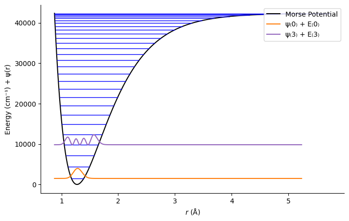
Plotting Morse Eigenfunctions#
The following code cell will plot a few of the Morse oscillator eigenfunctions for CO.
import numpy as np
from scipy.constants import h, hbar, c, u
from scipy.special import genlaguerre, gamma, factorial
import matplotlib.pyplot as plt

# Factor for conversion from cm⁻¹ to J
FAC = 100 * h * c

# ——— Utility Functions ———

def reduced_mass(mA, mB):
    """Return reduced mass (kg) for atoms of mass mA, mB in amu."""
    return mA * mB / (mA + mB) * u

def dissociation_energy(we, wexe):
    """Return De (J) from vibrational constants we, wexe in cm⁻¹."""
    return we**2 / (4 * wexe) * FAC

def morse_ke(we, mu):
    """Return effective spring constant ke (kg·s⁻²)."""
    return (2 * np.pi * c * 100 * we)**2 * mu

def morse_a(we, mu, De):
    """Return Morse parameter a (m⁻¹)."""
    return we * np.sqrt(2 * mu / De) * np.pi * c * 100

def morse_lambda(mu, De, a):
    """Return λ = sqrt(2µDe)/(aħ)."""
    return np.sqrt(2 * mu * De) / (a * hbar)

def vmax(lam):
    """Maximum bound-state quantum number."""
    return int(np.floor(lam - 0.5))

def make_rgrid(re, a, n=1000, f=0.999):
    """
    Build an r–grid (m) from rmin to rmax where V(rmin)=De and V(rmax)=f·De.
    Returns (r_array, dr).
    """
    rmin = re - np.log(2) / a
    rmax = re - np.log(1 - f) / a
    return np.linspace(rmin, rmax, n, retstep=True)

def morse_potential(r, De, a, re):
    """Morse potential V(r) in joules."""
    return De * (1 - np.exp(-a * (r - re)))**2

def energy_morse_J(v, we, wexe):
    """Morse oscillator level E_v in joules."""
    vp = v + 0.5
    return (we * vp - wexe * vp**2) * FAC

def turning_points(E, De, a, re):
    """Classical turning points (rm, rp) at energy E (J)."""
    b = np.sqrt(E / De)
    rm = re - np.log(1 + b) / a
    rp = re - np.log(1 - b) / a
    return rm, rp

def morse_wavefunction(v, r, lam, a, re, norm_peak=1.0):
    """
    Unnormalized Morse wavefunction ψ_v(r), scaled to `norm_peak`.
    Returns ψ(r).
    """
    z = 2 * lam * np.exp(-a * (r - re))
    alpha = 2 * (lam - v) - 1
    L = genlaguerre(v, alpha)
    psi = (z**(lam - v - 0.5) * np.exp(-z/2) * L(z))
    # scale to peak value norm_peak
    return psi * (norm_peak / np.max(np.abs(psi))) / 30

# ——— Example: CO molecule ———

# Input data
mA, mB    = 1.0, 35.0          # masses (amu)
we, wexe  = 2990.945, 52.818595 # vibrational constants (cm⁻¹)
re, Te    = 1.27455e-10, 0.0   # equilibrium bond length (m), electronic energy (arbitrary zero)

# Derived parameters
mu   = reduced_mass(mA, mB)
De   = dissociation_energy(we, wexe)
ke   = morse_ke(we, mu)
a    = morse_a(we, mu, De)
lam  = morse_lambda(mu, De, a)
v_max = vmax(lam)

# Build grid and compute potential
r, dr = make_rgrid(re, a)
V = morse_potential(r, De, a, re)

# ——— Plotting ———

fig, ax = plt.subplots(figsize=(8,5))

# Morse potential (converted back to cm⁻¹ for plotting + Te offset)

ax.plot(r*1e10, V/FAC + Te, color='black', label='Morse Potential')

if v_max > 1000:
    v_max = 10

# Energy levels and turning points
for v in range(v_max + 1):
    E = energy_morse_J(v, we, wexe)
    rm, rp = turning_points(E, De, a, re)
    ax.hlines(E/FAC + Te, rm*1e10, rp*1e10,
              colors='blue', linewidth=1)

# Plot two selected wavefunctions (v=0 and v=3)
for v, color in [(0, 'tab:orange'), (3, 'tab:purple')]:
    psi = morse_wavefunction(v, r, lam, a, re, norm_peak=we/2)
    psi_plot = psi ** 2 + energy_morse_J(v, we, wexe)/FAC + Te
    ax.plot(r*1e10, psi_plot, color=color, label=f'ψ₍{v}₎ + E₍{v}₎')

# Formatting
ax.set_xlabel(r'$r$ (Å)')
ax.set_ylabel(r'Energy (cm⁻¹) + ψ(r)')
ax.spines['top'].set_visible(False)
ax.spines['right'].set_visible(False)
ax.legend(loc='upper right')
plt.show()
Reflection: Symmetry of the Vibrational Probability Density#
Consider the probability density
$\(
|\psi_n(r)|^2
\)$
for the Morse‐oscillator eigenstates you just plotted.
Symmetry Question:
Is the probability density \(|\psi_n(r)|^2\) symmetric about the equilibrium bond length \(r_{eq}\)?
How does this compare to the harmonic oscillator eigenstates you studied earlier?
Physical Interpretation:
If the probability density is not perfectly symmetric, what physical feature of the Morse potential causes this asymmetry?
How does anharmonicity influence the shape and location of the vibrational wavefunction peaks?
Take a moment to sketch or describe qualitatively what you expect for \(|\psi_0(r)|^2\) and \(|\psi_1(r)|^2\) in the Morse model, and compare with the harmonic oscillator case.
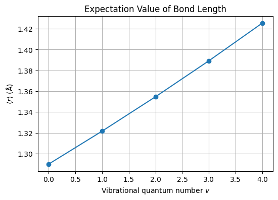
# ——— Expectation values ⟨r⟩ for v = 0…4 ———

states = range(5)
expectation_r = []

for v in states:
    # get the (unnormalized) wavefunction on the same grid
    psi = morse_wavefunction(v, r, lam, a, re)
    prob = psi**2

    # normalize
    norm = np.trapz(prob, r)
    prob_norm = prob / norm

    # compute ⟨r⟩
    exp_r = np.trapz(r * prob_norm, r)
    expectation_r.append(exp_r * 1e10)  # convert to Å

# ——— Plot ⟨r⟩ vs v ———

fig, ax = plt.subplots(figsize=(6,4))
ax.plot(states, expectation_r, marker='o', linestyle='-')
ax.set_xlabel('Vibrational quantum number $v$')
ax.set_ylabel(r'$\langle r \rangle$ (Å)')
ax.set_title('Expectation Value of Bond Length')
ax.grid(True)
plt.show()
🌉 Quantum Tunneling in the Morse Potential#
You will use the code below to compute probability density of the ground vibrational state of CO within the Morse oscillator model, which you will then use to compute the tunneling probability associated with the ground state.
Recall that the tunneling probability can computed as:
where \(r_{tp,l}\) is the left turning point and \(r_{tp, r}\) is the right turning point.
🧭 Question#
Use the code output to report the classical turning points \( r_{tp,l} \) and \( r_{tp,r} \) for the ground state.
Compute the probability of tunneling to the right of \(r_{tp,r}\)
P_tunneling_right, which integrates the probability density beyond \( r_{tp,r} \).What is the numerical value of this tunneling probability?
Is it significant compared to the total probability (≈1)?
Compute the probability of tunneling to the left of \(r_{tp,l}\)
P_tunneling_left, which integrates the probability density below \( r_{tp,l} \).What is the numerical value of this tunneling probability?
Is it significant compared to the total probability (≈1)?
How would you expect this tunneling probability to the right change for higher vibrational quantum numbers \( v > 0 \)? Why?
🧩 Guided Exercise: Tunneling Probability for the Ground State of CO#
In this activity, you will compute the tunneling probability for the ground vibrational state of a Morse oscillator representing CO.
The code below provides the basic setup of the molecule and Morse parameters.
Your task will be to:
Compute the classical turning points for ( v = 0 ),
Identify the forbidden region (( r > r_{tp,r} )),
Integrate the probability density in this region to estimate the tunneling probability.
A number of helper functions, including def turning_points(E, De, a, re):, are provided to compute the left and right turning points for a given state with energy E and a potential defined by De, a, and re. (The parameter a is equivalent to the parameter \(\beta\) from our notes).
Run the cell below to compute the value of these parameters.
import numpy as np
from scipy.constants import h, hbar, c, u
from scipy.special import genlaguerre, gamma, factorial
import matplotlib.pyplot as plt

# Factor for conversion from cm⁻¹ to J
FAC = 100 * h * c

# ——— Utility Functions ———

def reduced_mass(mA, mB):
    """Return reduced mass (kg) for atoms of mass mA, mB in amu."""
    return mA * mB / (mA + mB) * u

def dissociation_energy(we, wexe):
    """Return De (J) from vibrational constants we, wexe in cm⁻¹."""
    return we**2 / (4 * wexe) * FAC

def morse_ke(we, mu):
    """Return effective spring constant ke (kg·s⁻²)."""
    return (2 * np.pi * c * 100 * we)**2 * mu

def morse_a(we, mu, De):
    """Return Morse parameter a (m⁻¹)."""
    return we * np.sqrt(2 * mu / De) * np.pi * c * 100

def morse_lambda(mu, De, a):
    """Return λ = sqrt(2µDe)/(aħ)."""
    return np.sqrt(2 * mu * De) / (a * hbar)

def vmax(lam):
    """Maximum bound-state quantum number."""
    return int(np.floor(lam - 0.5))


def make_rgrid(re, a, n=1000, f=0.999):
    """
    Build an r–grid (m) from rmin to rmax where V(rmin)=De and V(rmax)=f·De.
    Returns (r_array, dr).
    """
    rmin = re - np.log(2) / a
    rmax = re - np.log(1 - f) / a
    return np.linspace(rmin, rmax, n, retstep=True)


def energy_morse_J(v, we, wexe):
    """Morse oscillator level E_v in joules."""
    vp = v + 0.5
    return (we * vp - wexe * vp**2) * FAC

def turning_points(E, De, a, re):
    """Classical turning points (rm, rp) at energy E (J)."""
    b = np.sqrt(E / De)
    rm = re - np.log(1 + b) / a
    rp = re - np.log(1 - b) / a
    return rm, rp

def morse_wavefunction(v, r, lam, a, re, norm_peak=1.0):
    """
    Unnormalized Morse wavefunction ψ_v(r), scaled to `norm_peak`.
    Returns ψ(r).
    """
    z = 2 * lam * np.exp(-a * (r - re))
    alpha = 2 * (lam - v) - 1
    L = genlaguerre(v, alpha)
    psi = (z**(lam - v - 0.5) * np.exp(-z/2) * L(z))
    # scale to peak value norm_peak
    return psi * (norm_peak / np.max(np.abs(psi))) / 30


# ——— Example: CO molecule ———

# Input data
mA, mB    = 1.0, 35.0          # masses (amu)
we, wexe  = 2990.945, 52.818595 # vibrational constants (cm⁻¹)
re, Te    = 1.27455e-10, 0.0   # equilibrium bond length (m), electronic energy (arbitrary zero)

# Derived parameters
mu   = reduced_mass(mA, mB)
De   = dissociation_energy(we, wexe)
ke   = morse_ke(we, mu)
a    = morse_a(we, mu, De)
lam  = morse_lambda(mu, De, a)
v_max = vmax(lam)

# Build grid for the wavefunction and probability density
r, dr = make_rgrid(re, a)

# define quantum number for ground state
v = 0

# compute psi_v
psi_v = morse_wavefunction(v, r, lam, a, re)

# compute P_v = psi_v^* psi_v
P_v = psi_v ** 2

# compute normalization constant based on area under P_v
norm = np.trapz(P_v, r)

# normalized probability density
P_v_norm = P_v / norm

# get E for v = 0
E = energy_morse_J(v, we, wexe)
Step 1: Complete the following block of code to compute the classical turning points#
The values of E, De, a, and re have been assigned by the previous block; utilize the
turning_points(E, De, a, re) function to assign the values of rtp_l, rtp_r below.
# TODO: Compute classical turning points
# Use the provided helper function turning_points(E, De, a, re)
# and print their values in meters.

rtp_l, rtp_r = ???

print(f" Left turning point:  {rtp_l:.4e} m")
print(f" Right turning point: {rtp_r:.4e} m")
 Left turning point:  1.1763e-10 m
 Right turning point: 1.3932e-10 m
Step 2: Integrate the probability density over the range of r outside of rtp_l and rtp_r#
We can integrate the (normalized) probability density P_v_norm with respect to r by using numpy’s trapz method, which implements the trapezoid rule to approximate an integral.
integraded_P = np.trapz(P_v_norm, r)
where this will integrate over all values of r, which should give us 1 by definition of normalized probability density!
We would like to apply the same approach to only the tunneling region. We can use the np.where() method to find the indices of all
values of the r array that are less than or equal to rtp_l, and we can use this function a second time to find the indices of all values
of the r array that are greater than or equal to rtp_r. This will allow us to use the np.trapz() method on only the slice of the
probability density that corresponds to the tunneling regions.
The syntax for the left tunneling region is shown in this Markdown block; implement this syntax in the following code cell and also apply it to the right tunneling region to complete the question.
# get all indices of r values <= rtp_l and store to l_idx
l_idx = np.where(r <= rtp_l)

# get the slice of r values to the left of rtp_l
r_left = r[l_idx]

# get the slice of P_v_norm values to the left of rtp_l
P_v_left = P_v_norm[l_idx]

# compute integral of the probability density on the slice of values to the left of rtp_l
P_tunneling_left = np.trapz(P_v_left, r_left)
# TODO: get all indices of r values <= rtp_l and store to l_idx
l_idx = ???

# TODO: get the slice of r values to the left of rtp_l
r_left = ???

# TODO: get the slice of P_v_norm values to the left of rtp_l
P_v_left = ???

# TODO: get all indices of r values >= rtp_l and store to r_idx
r_idx = ???

# TODO: get the slice of r values to the right of rtp_r
r_right = ???

# TODO: get the slice of P_v_norm values to the right of rtp_lr
P_v_right = ???


# Integrate the probability density on the left of rtp_l
P_tunneling_left = ???

# Integrate the probability density on the right of rtp_r
P_tunneling_right = ???

print(f" Probability of tunneling on left  side: {P_tunneling_left:.4e}")
print(f" Probability of tunneling on right side: {P_tunneling_right:.4e}")
import numpy as np
import matplotlib.pyplot as plt

# Compute ⟨r⟩ and corresponding energies for v = 0…4
states = range(10)
expectation_r = []
harmonic_expectation_r = []
expectation_E = []
print(F" re is {re}")
for v in states:
    # get wavefunction on grid
    psi = morse_wavefunction(v, r, lam, a, re)
    prob = psi**2
    # normalize
    prob /= np.trapz(prob, r)
    # expectation ⟨r⟩ (convert to Å)
    exp_r = np.trapz(r * prob, r) * 1e10
    expectation_r.append(exp_r)
    # energy level in cm⁻¹ plus Te
    Ev = energy_morse_J(v, we, wexe) / FAC + Te
    expectation_E.append(Ev)
    harmonic_expectation_r.append(re * 1e10)

# Now plot everything
fig, ax = plt.subplots(figsize=(8,5))

# 1. Morse potential (black)
ax.plot(r*1e10, V/FAC + Te, color='black', label='Morse Potential')

# 2. Energy levels (blue lines)
for v in range(12):
    E = energy_morse_J(v, we, wexe)
    rm, rp = turning_points(E, De, a, re)
    ax.hlines(E/FAC + Te, rm*1e10, rp*1e10,
              colors='blue', linewidth=1)

# 3. Two example wavefunctions (v=0,3)
for v, color in [(0, 'tab:orange'), (3, 'tab:purple')]:
    psi = morse_wavefunction(v, r, lam, a, re, norm_peak=we/2)
    psi_plot = psi**2 + energy_morse_J(v, we, wexe)/FAC + Te
    ax.plot(r*1e10, psi_plot, color=color, label=f'ψ₍{v}₎ + E₍{v}₎')

# 4. Expectation values ⟨r⟩ as red dots
ax.scatter(expectation_r, expectation_E,
           color='red', s=50, zorder=5,
           label=r'$\langle r\rangle$')
ax.scatter(harmonic_expectation_r, expectation_E,
           color='blue', s=30, zorder=5,
           label=r'$\langle r\rangle_{harmonic}$')

# Formatting
ax.set_xlabel(r'$r$ (Å)')
ax.set_ylabel(r'Energy (cm⁻¹) + ψ(r)')
ax.spines['top'].set_visible(False)
ax.spines['right'].set_visible(False)
ax.legend(loc='upper right')
plt.show()
Reflection: Comparing ⟨r⟩ in Harmonic vs. Morse Oscillators#
Take a moment to think about how the expectation value of the bond length, ⟨r⟩, changes as you go to higher vibrational states in each model.
Harmonic Oscillator
What is the qualitative behavior of ⟨r⟩ as you increase the quantum number (v)?
Why does a purely quadratic potential lead to that trend?
Morse Oscillator
How does the anharmonicity of the Morse potential modify the growth of ⟨r⟩ with (v)?
At high (v), how does ⟨r⟩ reflect the finite dissociation limit of the bond?
Comparison & Implications
In which regime (low vs. high (v)) do the two models agree most closely, and why?
How might differences in ⟨r⟩ affect predictions of spectroscopic transitions or bond dissociation?
Use these questions to guide a short discussion or to prompt your own notes on the physical significance of ⟨r⟩ in anharmonic versus harmonic vibrational models.
Transition State Optimization#
In addition to frequency information, vibrational analysis can be used to confirm whether a stationary point that has been identified via a geometry optimization is a minimum in all of the coordinates, a transition state, or some other high-order saddle point. Each of these cases can be differentiated by the number of imaginary frequencies that result from the vibrational analysis. Recall that the harmonic frequency is related to the square root of the second derivative of the potential along one of the normal modes. If the potential is a minimum along this coordinate, then the second derivative is positive, and the frequency is real (because the square root of a positive number is real-valued). If the potential is a maximum along this coordinate, then the second derivative is negative, and the frequency is imaginary (because the square root of a negative number is imaginary). Hence, if all of the frequencies obtained from the vibrational analysis are real, then the molecule is at a minimum all of coordinates. If there exists one and only one imaginary frequency, then the molecule is at a transition state. If there are multiple imaginary fruequencies, then the molecule is at some high-order saddle point that is not a transition state.
Consider the following simple isomerization reaction:
The transition state for this reaction should be found at an H-C-N bond angle of roughly 70\(\degree\). The following code will identify this transition state and perform a frequency analysis on the optimized structure.
Note This example involves using another open-source quantum chemistry package, Psi4. This can be installed on Mac and Linux systems with relative ease, but cannot be installed in a Google Colab environment like PySCF can. You may utilize the free, web-based ChemCompute server to run this calculation.
import psi4
import numpy as np
# set molecule
mol = psi4.geometry("""
h
c 1 1.2
n 2 1.2 1 70.0
symmetry c1
""")

# set some options for psi4.
# don't forget to specify the transition state search
psi4.set_options({'basis': 'cc-pvdz',
                  'guess_mix': True,
                  'reference': 'uhf',
                  'opt_type': 'ts'})

# tell psi4 not to print any output to the screen
psi4.core.be_quiet()

# optimize geometry
psi4.optimize('scf')

# calculate harmonic frequencies
en, wfn = psi4.frequency('scf', return_wfn = True)

# extract frequencies from the wave function
freq = np.asarray(wfn.frequencies())
for i in range(len(freq)):
    print('The harmonic frequency for mode %i is %8.1f cm^-1' % (i, freq[i]) )