Chapter 3: Translational Motion

Prof. Eugene DePrince, Florida State University and Prof. Jay Foley, UNC Charlotte

This notebook develops solutions to the time-independent Schrödinger equation (TISE) for several translational problems (e.g., particle-in-a-box, tunneling through a one-dimensional barrier, etc.). Relevant Python code is provided to assist in visualizing the wave functions and obtaining numerical solutions to the TISE.

The Free Particle

The Wave Function and Its Properties

Consider the Hamiltonian for particle moving in one dimension (1D)

\[\begin{align} \hat{H} = \hat{T}_x + \hat{V}(x) \end{align}\]

In the free particle problem, the particle is subject to no external forces, which means that the potential term, \(\hat{V}(x)\), vanishes, so

\[\begin{align} \hat{H} = \hat{T}_x = -\frac{\hbar^2}{2m}\frac{d^2}{dx^2} \end{align}\]

Like the other Hamiltonians that will be considered in this notebook, this Hamiltonian does not depend on time. As a result, we can solve the time-independent Schrödinger equation for the spatial part of the wave function, \(\psi(x)\),

\[\begin{split}\begin{align} \hat{H} \psi(x) &= E \psi(x) \\ -\frac{\hbar^2}{2m}\frac{d^2}{dx^2} \psi(x) &= E \psi(x)\\ \end{align}\end{split}\]

Rearranging the constants, we have

\[\begin{split}\begin{align} \frac{d^2}{dx^2} \psi(x) &= -\frac{2mE}{\hbar^2} \psi(x)\\ &= -k^2 \psi(x) \end{align}\end{split}\]

where we have introduced a constant, \(k = +(2mE/\hbar^2)^{1/2}\). Now, we have two useful pieces of information:

1. The wave function should be an eigenfunction of \(\frac{d^2}{dx^2}\) (e.g., exponential, sin, or cosine functions)

2. The wave function should have a negative eigenvalue.

A general form for \(\psi(x)\) that satisfies both of these requirements is

\[\begin{align} \psi(x) = A e^{ikx} + B e^{-ikx} \end{align}\]

Let’s verify that this form satisfies the Schrödinger equation

\[\begin{split}\begin{align} \hat{H}\psi(x) &= -\frac{\hbar^2}{2m} \frac{d^2}{dx^2} \left [ A e^{ikx} + B e^{-ikx} \right ] \\ &= ik \left ( -\frac{\hbar^2}{2m} \right ) \frac{d}{dx} \left [ A e^{ikx} + B e^{-ikx} \right ] \\ &= (ik)^2 \left ( -\frac{\hbar^2}{2m} \right ) \frac{d}{dx} \left [ A e^{ikx} + B e^{-ikx} \right ] \\ &= -k^2 \left ( -\frac{\hbar^2}{2m} \right ) \psi(x) \\ &= \frac{k^2\hbar^2}{2m} \psi(x) \end{align}\end{split}\]

So, yes, \(\psi(x) = Ae^{ik} + Be^{-ikx}\) is an eigenfunction of the Hamiltonian for a free particle moving in one dimension, and

\[\begin{align} E = \frac{k^2\hbar^2}{2m} \end{align}\]

is the associated eigenvalue. We can draw one interesting conclusion from this result: nothing limits the value that \(k\) can take (as long as it is real-valued). As a result, the energy of a free particle is not quantized.

Question: Physical Meaning of \(e^{\pm ikx}\) and Operator Eigenfunctions

What do the terms \(e^{\pm ikx}\) mean, physically?

Let’s assume that \(B = 0,\) so \(\psi(x) = Ae^{ikx}\).
This function is still an eigenfunction of the Hamiltonian, with the same eigenvalue.

Question:
Is \(\psi(x)\) also an eigenfunction of any other operators, like the momentum operator \(\hat{p}_x\)?

Try computing \(\hat{p}_x \psi(x)\) by hand.
Then click below to reveal the full worked-out solution.

Click to reveal the solution

We apply the momentum operator to \(\psi(x) = A e^{ikx}\):

\[\begin{split} \begin{align} \hat{p}_x \psi(x) &= -i\hbar \frac{d}{dx} (Ae^{ikx}) \\ &= -i\hbar \cdot i k A e^{ikx} \\ &= \hbar k \psi(x) \end{align} \end{split}\]

✅ So, yes! \(\psi(x)\) is an eigenfunction of \(\hat{p}_x\), with eigenvalue \(\hbar k\).

This result indicates that the state described by this function has a well-defined (or definite) value of the momentum in the \(x\)-direction. Recall, \(k = +\left ( \frac{2mE}{\hbar^2} \right )^{1/2},\) so, \(k \ge 0\) and \(\hbar k \ge 0\), which implies that \(p_x \ge 0\). Since the momentum of the particle is positive and well-defined, the state described by \(\psi(x) = Ae^{ikx}\) corresponds to the case where the free particle is traveling in the \(+x\) direction, with momentum \(\hbar k\). If this interpretation is not clear, recall the following

1. Any function can be expanded in terms of eigenfunctions of a Hermitian operator, \(\hat{B}\), as \(\psi = \sum_i c_i g_i\) where \(\hat{B} g_i = b_i g_i\)

2. Any measurement of \(B\) results in one of the eigenvalues, \(b_i\). The probability with which we observe \(b_i\) is proportional to \(|c_i|^2\). The proportionality becomes an equality of the wave function is normalized.

3. If \(\psi\) is exactly equal to an eigenfunction of \(\hat{B}\), then there is only one term in the sum above, and the only value of \(B\) that would ever be observed would be the corresponding eigenvalue. In the case above, we have \(\psi(x) = A e^{ikx}\), which we showed is an eigenfunction of \(\hat{p}_x\).

We obtain a similar result if we start from the free particle wave function and assume that \(A = 0\). In this case, \(\psi(x) = B e^{-ikx}\) is also an eigenfunction of \(\hat{p}_x\), but the associated eigenvalue is \(-\hbar k\). Hence, \(\psi(x) = Be^{-ikx}\) represents a state where the particle has definite value of the momentum, \(-\hbar k\) (moving in the \(-x\) direction).

More Practice:
Show \(\psi(x) = B e^{-ikx}\) is also an eigenfunction of \(\hat{p}_x\) with eigenvalue \(-\hbar k\).

Try computing \(\hat{p}_x \psi(x)\) by hand.
Then click below to reveal the full worked-out solution.

Click to reveal the solution

We apply the momentum operator to \(\psi(x) = B e^{-ikx}\):

\[\begin{split} \begin{align} \hat{p}_x \psi(x) &= -i\hbar \frac{d}{dx} (Be^{-ikx}) \\ &= -i\hbar \cdot -i k B e^{-ikx} \\ &= -\hbar k \psi(x) \end{align} \end{split}\]

✅ So, yes! \(\psi(x) = B e^{-ikx}\) is an eigenfunction of \(\hat{p}_x\), with eigenvalue \(-\hbar k\).

Question: Is the General Free Particle an Eigenfunction of Momentum?

The general form of the free-particle wave function is:

\[ \psi(x) = A e^{ikx} + B e^{-ikx} \]

This is a superposition of two pure-momentum states.
Is \(\psi(x)\) an eigenfunction of the momentum operator \(\hat{p}_x\)?

Choose one:

A. Yes, because \(\hat{p}_x \psi(x) = \hbar k \psi(x)\)
B. No, because it includes both positive and negative momentum components
C. Yes, as long as \(|A|^2 + |B|^2 = 1\)
D. No, because the Hamiltonian doesn’t have momentum as an observable

Click to reveal the solution

We apply the momentum operator:

\[\begin{split} \begin{align} \hat{p}_x (A e^{ikx} + B e^{-ikx}) &= \hat{p}_x A e^{ikx} + \hat{p}_x B e^{-ikx} \\ &= \hbar k A e^{ikx} - \hbar k B e^{-ikx} \\ &= \hbar k (A e^{ikx} - B e^{-ikx}) \end{align} \end{split}\]

Note the minus sign in the second term:
\(\psi(x)\) is not an eigenfunction of \(\hat{p}_x\), since the result is not proportional to the original wave function.

Instead, \(\psi(x)\) is a superposition of two momentum eigenfunctions, one with momentum \(+\hbar k\) and one with \(-\hbar k\).
The probability of measuring the particle with momentum \(+\hbar k\) is proportional to \(|A|^2\),
and for \(-\hbar k\) it is proportional to \(|B|^2\).

✅ Correct answer: B

Question: Is \(\psi(x) = Ae^{ikx}\) an Eigenfunction of the Position Operator?

We’ve seen that \(\psi(x) = A e^{ikx}\) is an eigenfunction of the momentum operator.
But what about position?

Let’s test whether \(\psi(x)\) is an eigenfunction of the position operator \(\hat{x}\) by applying the operator directly.
Then, try computing the expectation value \(\langle x \rangle\) for this wave function.

Does the particle have a well-defined position?
What can you say about where the particle is likely to be found?

Click to reveal the solution

We apply the position operator to the wave function:

\[ \hat{x} \psi(x) = x \cdot \psi(x) = A x e^{ikx} \]

This is not proportional to the original wave function \(A e^{ikx}\),
so \(\psi(x)\) is not an eigenfunction of the position operator.

---

Now let’s calculate the expectation value of position:

\[ \langle x \rangle = \frac{\langle \psi(x) | x | \psi(x) \rangle}{\langle \psi(x) | \psi(x) \rangle} \]

Plug in the expression for \(\psi(x) = A e^{ikx}\):

\[ \langle x \rangle = \frac{|A|^2 \int_{-\infty}^{\infty} e^{-ikx} \, x \, e^{ikx} \, dx}{|A|^2 \int_{-\infty}^{\infty} e^{-ikx} e^{ikx} \, dx} = \frac{\int_{-\infty}^{\infty} x \, dx}{\int_{-\infty}^{\infty} dx} \]

The numerator and denominator are both divergent, but their ratio is symmetric around \(x = 0\),
so by symmetry arguments (or via regularization), we get:

\[ \langle x \rangle = 0 \]

---

🔍 Interpretation:
This result doesn’t mean the particle is always at \(x = 0\), but rather that, on average, measurements would be equally likely to yield positions on either side of the origin.
The wave function is completely delocalized — we have no knowledge of where the particle is, only that the average position is zero.

The Born interpretation of the wave function provides a result consistent with this one. The probability density

\[\begin{align} |\Psi(x)|^2 = |A|^2 e^{-ikx} e^{ikx} = |A|^2 \end{align}\]

is equal to a constant over all space, which implies we’re equally likely to find the particle anywhere in \(x\). Put another way, we have no idea where the particle will be located before a measurement is taken.

Heisenberg Uncertainty Principle

This result is a specific manifestation of Heisenberg’s Uncertainty Principle. It is impossible to specify, with arbitrary precision, both the position and momentum of a quantum mechanical particle. The wave function \(\psi(x) = A e^{ikx}\) represents a state with a well-defined value for the momentum, meaning we know exactly what the momentum is for the particle in this state. As a consequence, we cannot know anything about the position of the particle.

Mathematically, we have

\[\begin{align} \Delta x \Delta p_x \ge \frac{1}{2}\hbar \end{align}\]

where \(\Delta \Omega\) represents the uncertainty in the observable \(\Omega\). The uncertainty is calculated as the standard deviation

\[\begin{align} \Delta \Omega = \left ( \langle \Omega^2 \rangle - \langle \Omega \rangle^2 \right )^{1/2} \end{align}\]

The uncertainty relationship between position and momentum is a consequance of the particle-wave duality of microscopic particles. See this page for a graphical illustration of this concept.

Let’s calculate the uncertainty in position and momentum for the state represented by the wave function \(\psi(x) = A e^{ikx}\). Because \(\psi(x)\) is an eigenfunction of the momentum operator, we immediately know that

\[\begin{split}\begin{align} \langle p_x \rangle &= \hbar k \\ \langle p_x^2 \rangle &= \hbar^2 k^2 \end{align}\end{split}\]

In the second line, we take advantage of the fact that an eigenfunction of an operator \(\hat{B}\) is also an eigenfunction of the operator \(\hat{B}^2\). Now, the uncertainty in the momentum is

\[\begin{split}\begin{align} \Delta p_x =& \left ( \langle p_x^2 \rangle - \langle p_x \rangle^2 \right )^{1/2} \\ &= \left( \hbar^2 k^2 - \hbar^2 k^2 \right )^{1/2} \\ &= 0 \end{align}\end{split}\]

Note that, in general, a variance / standard deviation of zero for a given property implies that the state is an eigenfunction of the operator associated with that observable.

Now, consider the uncertainty in \(x\),

\[\begin{align} \Delta x =& \left ( \langle x^2 \rangle - \langle x \rangle^2 \right )^{1/2} \end{align}\]

We showed already that \(\langle x \rangle = 0\). Next, we have

\[\begin{split}\begin{align} \langle x^2 \rangle &= \frac{\langle \psi(x)|x^2|\psi(x)\rangle}{\langle \psi(x) | \psi(x) \rangle} \\ &= \frac{|A|^2\int_{-\infty}^{\infty} e^{-ikx} x^2 e^{ikx} dx}{|A|^2\int_{-\infty}^{\infty} e^{-ikx} e^{ikx} dx} \\ &= \frac{\int_{-\infty}^{\infty} x^2 dx}{\int_{-\infty}^{\infty} dx} \end{align}\end{split}\]

Both the numerator and denomator are integrals over even functions, which are infinite, but the numerator is a larger infinity and thus

\[\begin{align} \langle x^2 \rangle = \infty \end{align}\]

and

\[\begin{align} \Delta x = \infty \end{align}\]

Hence, there is an infinite uncertainty in the position of the particle represented by the state, \(\psi(x) = A e^{ikx}\). This result is consistent with the Born interpretation of the state suggesting that one would be equally likely to find the particle anywere, and, thus, we have no idea where the particle is without taking a measurement.

More generally, the Heisenberg Uncertainty Principle applies to other pairs of observables, \(A\) and \(B\). Specifically, the product of uncertainties in \(A\) and \(B\) are bounded by

\[\begin{align} \Delta A \Delta B \ge \frac{1}{2} |\langle [\hat{A}, \hat{B}]\rangle| \end{align}\]

If \(\hat{A}\) and \(\hat{B}\) commute, then

\[\begin{align} \Delta A \Delta B \ge 0 \end{align}\]

which suggests that it would be possible for states to exist where the uncertainties in \(A\) and \(B\) are both zero. On the other hand, if \(\hat{A}\) and \(\hat{B}\) do not commute, then there is some finite lower bound to the degree to which \(A\) and \(B\) can be known simultaneously.

If \([\hat{A}, \hat{B}] = 0\) and \(\Delta A\) and \(\Delta B\) are both zero, then the state would be an eigenfunction of both \(\hat{A}\) and \(\hat{B}\), which brings us to a theorem

Theorem: If Hermitian operators \(\hat{A}\) and \(\hat{B}\) commute, then there exists a common, complete set of eigenfunctions of these operators.

Stated another way, if \(\hat{A}\) and \(\hat{B}\) have a common, complete set of eigenfunctions, then they must commute.

Proof

Consider linear Hermitian operators \(\hat{A}\) and \(\hat{B}\) that share a common set of eigenfunctions:

\[\begin{split}\begin{align} \hat{A} g_i &= a_i g_i \\ \hat{B} g_i &= b_i g_i \end{align}\end{split}\]

Now, consider a general function, \(f\), that is expanded in terms of these functions, \(\{g_i\}\), which form a complete set

\[\begin{align} f = \sum_k c_k g_k \end{align}\]

Let us evaluate how the commutator of \(\hat{A}\) and \(\hat{B}\) act on this function

\[\begin{split}\begin{align} [\hat{A}, \hat{B}]f &= [\hat{A}, \hat{B}]\sum_k c_k g_k \\ &= (\hat{A}\hat{B} -\hat{B}\hat{A})\sum_k c_k g_k\\ &= \sum_k c_k \left [ \hat{A} (\hat{B}g_k) - \hat{B}(\hat{A}g_k) \right ]\\ &= \sum_k c_k \left [ b_k \hat{A} g_k - a_k \hat{B} g_k \right ] \\ &= \sum_k c_k \left [ b_k a_k - a_k b_k \right ] g_k \\ [\hat{A}, \hat{B}]f &= 0 \end{align}\end{split}\]

Therefore \([\hat{A}, \hat{B}] = 0\).

If we can write down free-particle wave functions that are eigenfunctions of both the Hamiltonian and the momentum operator (i.e., \(\psi(x) = C e^{\pm ikx})\), then these operators must commute. Recall that the free-particle Hamiltonian is purely kinetic, and the kinetic energy operator can be expressed in terms of the momentum operator

\[\begin{align} \hat{H} = \hat{T} = \frac{\hat{p}_x^2}{2m} \end{align}\]

Now, it should be clear after this discussion that the commutator between this operator and the momentum operator should vanish. Indeed, it does,

\[\begin{split}\begin{align} [\hat{H}, \hat{p}_x] &= [\frac{\hat{p}_x^2}{2m}, \hat{p}_x] \\ &= \frac{1}{2m} [\hat{p}_x^2, \hat{p}_x] \\ &= 0 \end{align}\end{split}\]

because, as we learned in the last notebook, the commutator of any operator with any power of itself is zero.

Practice

Question 1: Derive the result

\[\Delta x \, \Delta p_x \ge \frac{1}{2} \hbar\]

using the general expression for Heisenberg’s Uncertainty principle:

\[\Delta x \, \Delta p_x \ge \frac{1}{2} \left| \langle [ \hat{x}, \hat{p}_x ] \rangle \right|\]

Answer 1

Let us first evaluate the commutator of \(\hat{x}\) and \(\hat{p}_x\):

\[[\hat{x}, \hat{p}_x]f = x\left(-i\hbar \frac{d}{dx}\right)f - \left(-i\hbar \frac{d}{dx}\right)xf\]

\[= -i\hbar x f' + i\hbar \left(f + x f'\right)\]

\[[\hat{x}, \hat{p}_x]f = i\hbar f\]

Therefore:

\[[\hat{x}, \hat{p}_x] = i\hbar\]

Now, insert this result into the expression for the joint uncertainty in \(x\) and \(p_x\):

\[\Delta x \, \Delta p_x \ge \frac{1}{2} \left| \langle i\hbar \rangle \right|\]

For the expectation value, we have:

\[\langle i\hbar \rangle = \frac{\langle \psi | i\hbar | \psi \rangle}{\langle \psi | \psi \rangle}\]

\[= i\hbar \frac{\langle \psi | \psi \rangle}{\langle \psi | \psi \rangle}\]

\[= i\hbar\]

For any non-zero wave function \(\psi\).

So:

\[\Delta x \, \Delta p_x \ge \frac{1}{2} | i\hbar |\]

\[= \frac{1}{2} \hbar\]

because:

\[|i\hbar| = \left[ (-i\hbar)(i\hbar) \right]^{1/2} = \left[ \hbar^2 \right]^{1/2} = \hbar\]

Infinite Square Well Potential, aka, Particle-in-a-box model

The particle-in-a-box (PIB) model describes a quantum mechanical particle confined within an infinite square well potential. While this model is simplified, it effectively captures qualitative trends in the electronic structure of molecular systems, particularly conjugated organic compounds.

Application to Conjugated Dye Molecules

The one-dimensional PIB model successfully predicts the red-shift in electronic excitation energies as the conjugation length of dye molecules increases. This correlation arises because the excitation energies of these systems are closely related to the HOMO-LUMO gap—the energy difference between the highest-occupied molecular orbital (HOMO) and lowest-unoccupied molecular orbital (LUMO). In conjugated dye systems, these correspond to the π and π* orbitals, respectively.

Why the PIB Model Works

The PIB model provides a good approximation for π → π* transitions in conjugated systems for several key reasons:

• Delocalization: The π electrons are delocalized across the entire conjugated backbone of the molecule

• Weak nuclear attraction: These electrons are relatively diffuse and experience weaker attraction to individual nuclei

• Reduced electron-electron repulsion: The delocalized nature minimizes strong repulsive interactions between electrons

Physical Interpretation

Essentially, the PIB model treats electrons as nearly free particles that are confined by infinite potential barriers at the boundaries of the conjugated system. The remarkable agreement between PIB predictions and experimental π-system energies suggests that conjugated π electrons behave, to a first approximation, like free electrons with spatial confinement—a testament to their delocalized, weakly-bound nature.

from IPython.display import Image
Image(url = "https://raw.githubusercontent.com/deprincelab/deprincelab.github.io/main/tutorials/jupyter_notebooks/translation/pib_red_shift.png")

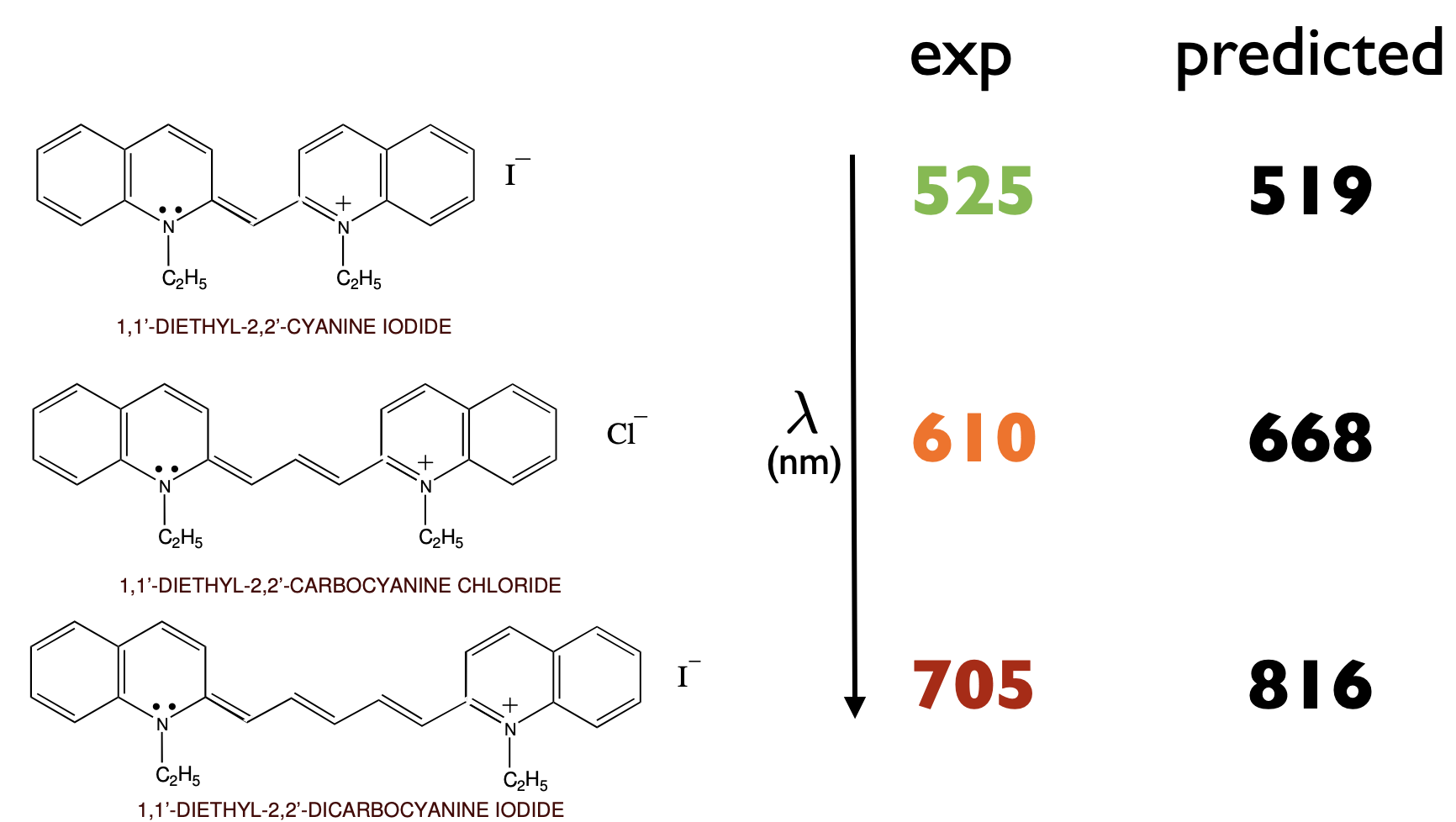
Obviously, the agreement with experiment is not great, but it is surprisingly good, given the crudeness of the model. As will be discussed below, particles (in the case above, electrons) feel no potential inside the “box” (the \(\pi\)-network of the dye molecules), despite the presence of the nuclei and other electrons.

One-Dimensional Particle-in-a-Box

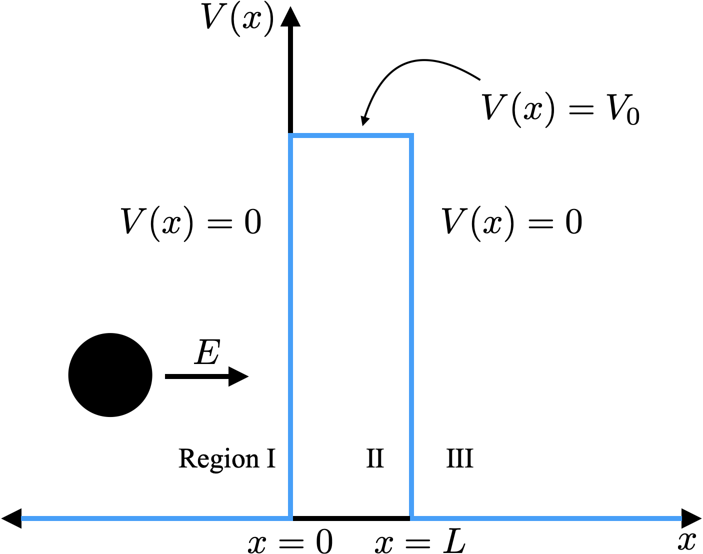
Consider a particle of mass, \(m\), that is moving in the \(x\)-direction and experiences an infinite square potential of width, \(L\). Graphically, this potential has the form:

Image(url = "https://raw.githubusercontent.com/deprincelab/deprincelab.github.io/main/tutorials/jupyter_notebooks/translation/infinite_square_well_potential.png")

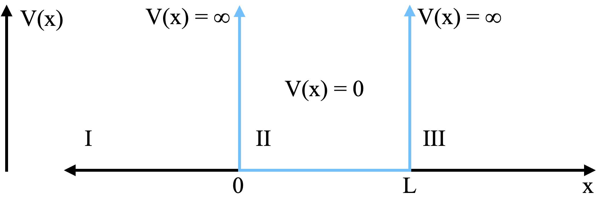
Mathematically, we define this potential in a piecewise way as

Region I:

\[\begin{align} V(x) = \infty\text{, }~~~x < 0 \end{align}\]

Region II:

\[\begin{align} V(x) = 0\text{, }~~~0 \le x \le L \end{align}\]

Region III:

\[\begin{align} V(x) = \infty\text{, }~~~x > L \end{align}\]

As such, the TISE should be solved in a piecewise way, i.e., for each region of space. We have

\[\begin{split}\begin{align} \psi(x) = \psi_I(x) ~~~ &\text{if } x < 0 \\ \psi(x) = \psi_{II}(x) ~~~ &\text{if } 0 \le x \le L \\ \psi(x) = \psi_{III}(x) ~~~ &\text{if } x > L \end{align}\end{split}\]

where \(\psi_I\), \(\psi_{II}\), and \(\psi_{III}\) satisfy

\[\begin{split}\begin{align} \hat{H} \psi_I(x) = E \psi_I(x) ~~~ &\text{if } x < 0 \\ \hat{H} \psi_{II}(x) = E \psi_{II}(x) ~~~ &\text{if } 0 \le x \le L \\ \hat{H} \psi_{III}(x) = E \psi_{III}(x) ~~~ &\text{if } x > L \end{align}\end{split}\]

To start, what does the wave function look like outside of the box (in regions I and III)? Consider the Schrödinger equation for region I:

\[\begin{split}\begin{align} \hat{H}\psi_I(x) &= E \psi_I \\ \left [ -\frac{\hbar^2}{2m}\frac{d^2}{dx^2} + V(x) \right ] \psi_I(x) &= E \psi_I(x) \\ -\frac{\hbar^2}{2m}\frac{d^2}{dx^2}\psi_I(x) &= [E-V(x)]\psi_I(x) \\ \frac{1}{V(x)-E}\frac{\hbar^2}{2m}\frac{d^2}{dx^2}\psi_I(x) &= \psi_I(x) \end{align}\end{split}\]

Recall that the potential is infinite in this region of space, so,

\[ \psi_I(x) = \lim_{V(x)\to \infty} \frac{1}{V(x)-E}\frac{\hbar^2}{2m}\frac{d^2}{dx^2}\psi_I(x) = 0\]

From this simple analysis, we can conlude that the wave function must go to zero as \(V(x)\) approaches infinity. Therefore the probability of finding a particle at \(x \le 0\) is zero (\(|\psi_I(x)|^2 = 0\)). This result makes sense because the particle would need infinite kinetic energy to overcome the infinite potential energy barrier required to enter that region of space.

A similar analysis for region III leads to

\[ \begin{align} \psi_{III}(x) = 0 \end{align}\]

In region II, the Schrödinger equation has a non-trivial solution. We have

\[\begin{split}\begin{align} \hat{H}\psi_{II}(x) &= E\psi_{II}(x) \\ -\frac{\hbar^2}{2m} \frac{d^2}{dx^2} \psi_{II}(x) &= -E\psi_{II}(x) \\ \frac{d^2}{dx^2} \psi_{II}(x) &= -\frac{2mE}{\hbar^2} \psi_{II}(x) \\ \frac{d^2}{dx^2} \psi_{II}(x) &= -k^2 \psi_{II}(x) \\ \end{align}\end{split}\]

with \(k = \left ( \frac{2mE}{\hbar^2} \right )^{1/2}\). Like the free-particle, a general solution to this differential equation is

\[\begin{align} \psi_{II}(x) = A e^{ikx} + B e^{-ikx} \end{align}\]

Unlike the free-particle problem, the probability amplitudes, \(A\) and \(B\), can be determined by considering the boundary conditions for the problem. These are the conditions that must be satisfied by the wave function in order for it to be well-behaved. Before applying these conditions, note that it will actually be easier to solve this problem by representing the wave function in terms of sine and cosine functions, as opposed to complex exponential functions. Euler’s formula can be used to express \(\psi_{II}\) in this way. We have

\[\begin{align} e^{\pm ikx} = \text{cos}(kx) + i \text{sin}(\pm kx) \end{align}\]

or

\[\begin{align} e^{\pm ikx} = \text{cos}(kx) \pm i \text{sin}(kx) \end{align}\]

Given this relationship, it is eash to show that

\[\begin{align} \psi(x) = (A+B) \text{cos}(kx) + i (A-B)\text{sin}(kx) \end{align}\]

or

\[\begin{align} \psi(x) = C \text{cos}(kx) + D \text{sin}(kx) \end{align}\]

where we have introduced new constant factors, \(C = A+B\) and \(D = i (A-B)\).

Now, what are \(C\) and \(D\)? As mentioned above, we can determine these constants by the application of boundary conditions. First, in order for \(\psi(x)\) to be well-behaved, it must be continuous over all space. In particular, it must be continuous at the edges of the box (at \(x=0\) and \(x=L\)), which places restrictions on \(\psi_{II}\), namely

\[\begin{align} \psi_{II}(x = 0) = \psi_{I}(x = 0) = 0 \end{align}\]

and

\[\begin{align} \psi_{II}(x = L) = \psi_{III}(x = L) = 0 \end{align}\]

For the first of these conditions, we have

\[\begin{split} \begin{align} 0 &= \psi_{II}(0) \\ &= C \text{cos}(0) + D \text{sin}(0) \\ &= C \end{align}\end{split}\]

and the wave function simplifies to

\[\begin{align} \psi_{II}(x) = D \text{sin}(kx) \end{align}\]

The second boundary condition gives us

\[\begin{align} 0 = \psi_{II}(L) = D \text{sin}(k L) \end{align}\]

This equation could be satisfied with the choice \(D = 0\), but then \(\psi(x)\) would be zero over all space, which means that \(|\psi(x)|^2 = 0\) over all space, implying that there is zero probability of finding the particle anywhere. We reject this unphysical solution. How else can this equation be satisfied? The sine function must be zero; the following Python code will visualize where this is the case:

import numpy as np
import matplotlib.pyplot as plt

# Generate x values from 0 to 6π
x = np.arange(0, 6*np.pi, 0.01)
sin_x = np.sin(x)

plt.figure()
plt.plot(x, sin_x)
plt.xlim(0, 6*np.pi)
plt.ylabel('sin(x)')
plt.xlabel('x')

# Set x-axis ticks at multiples of π
pi_ticks = np.arange(0, 7) * np.pi  # 0, π, 2π, 3π, 4π, 5π, 6π
pi_labels = ['0', 'π', '2π', '3π', '4π', '5π', '6π']

plt.xticks(pi_ticks, pi_labels)
plt.grid(True, alpha=0.3)  

plt.show()

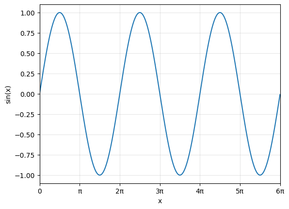
\(\text{sin}(x)\) is zero whenever \(x = n \pi\), where \(n\) is an integer. So, the boundary condition can be satisfied if \(kL = n\pi\), giving \(k = \frac{n\pi}{L}\) and

\[\begin{align} \psi_{II}(x) = D \text{sin}\left (\frac{n\pi x}{L}\right ) \end{align}\]

We have not yet determined the constant \(D\), but we did stumble upon an interesting result. Recall that \(k\) is related to the energy:

\[\begin{align} k = \left ( \frac{2 m E}{\hbar^2} \right )^{1/2} = \frac{n\pi}{L} \end{align}\]

Rearranging for the energy, we find

\[\begin{align} E_n = \frac{\hbar^2 n^2 \pi^2}{2 m L^2} \end{align}\]

or, since \(\hbar = \frac{h}{2\pi}\)

\[\begin{align} E_n = \frac{h^2 n^2}{8 m L^2} \end{align}\]

Here, we have added a subscript “\(n\)” to the symbol for the energy to denote that the energy for each state can be labeled by \(n\). Because \(n\) must be an integer, the energy for a PIB is quantized, which means that it can only take on certain values, and the quantization of the energy results from applying restrictions to the wave function. We call \(n\) a quantum number; this quantum number characterizes the state of the particle.

Are there any other restrictions on the value that \(n\) can take, aside from being an integer? Yes. First, consider the case where \(n=0\):

\[\begin{align} \psi_{II}^{n=0}(x) = D \text{sin} \left ( \frac{0 x \pi}{L} \right ) = 0 \end{align}\]

which would imply that the wave function is zero everywhere. We already rejected such a situation as unphysical earlier, and the do the same here. The case \(n=0\) is not allowed. What about \(n < 0\)? Let’s try \(n=-1\):

\[\begin{split} \begin{align} \psi_{II}^{n=-1}(x) &= D \text{sin} \left ( \frac{-1 x \pi}{L} \right ) \\ &= -D \text{sin} \left ( \frac{1 x \pi}{L} \right ) \\ &= \psi_{II}^{n=1}(x) \end{align}\end{split}\]

More generally,

\[\begin{align} \psi_{II}^{-n}(x) = -\psi_{II}^{n}(x) \end{align}\]

When introducing the concept of normalization in the last notebook, we discussed idea that two states that differ by only a multiplicative constant represent the same state. So, because the wave functions for \(n\) and \(-n\) differ by only a sign, they must represent the same state. For this reason, we ignore all \(n < 0\), because these states are redundant. Hence, the allowed values for \(n\) are all positive integers, 1, 2, 3, etc. The lowest-energy state (having \(n=0\)) is the “ground state.” All other PIB states have higher energy and are called “excited states.”

After applying two boundary conditions, we have yet to determine the constant \(D\). This constant can be determined by normalization:

\[\begin{split}\begin{align} \int_{-\infty}^{\infty} |\psi(x)|^2 dx &= 1 \\ &= \int_{0}^{L} |\psi_{II}(x)|^2 dx \end{align}\end{split}\]

because the integrals over \(|\psi(x)|^2\) in regions I and III are zero. Now,

\[\begin{split}\begin{align} 1 &= |D|^2 \int_0^L \text{sin}^2\left ( \frac{n \pi x}{L} \right ) dx \\ &= \frac{1}{2} D^2 \int_0^L \left [ 1 - \text{cos}\left ( \frac{2 n \pi x}{L}\right ) \right ] dx \\ &= \left . \frac{1}{2} D^2 \left [ x - \frac{L}{2\pi n}\text{sin}\left ( \frac{2 \pi n x}{L} \right ) \right ] \right|_0^L \\ &= \frac{1}{2}D^2 L\\ D &= \left ( \frac{2}{L} \right ) ^{1/2} \end{align}\end{split}\]

where, in the second line, we assumed that \(D\) is real-valued, and made use of the double angle formula \([2 \text{sin}^2(t) = 1 - \text{cos}(2t)].\) Now, we have fully defined the spatial wave function for the one-dimensional PIB problem:

\[\begin{split} \begin{align} \psi_n(x) &= \left ( \frac{2}{L} \right)^{1/2} \text{sin}\left ( \frac{n\pi x}{L}\right)\text{, if }~~~0 \le x \le L \\ &= 0\text{, }~~~\text{otherwise} \end{align}\end{split}\]

and the energy of the state represented by this wave function is \(E_n\).

Let’s visualize the wave functions and probability densities for the first few \(n\). For simplicity, we will take the particle to be an electron with mass, \(m = m_e\), and we will use atomic units, where \(\hbar = 1\) and \(m_e = 1\). The length of the box will be \(L = 1 a_0\).

L = 1.0
hbar = 1.0
m = 1.0

x = np.arange(0, L, 0.01)

wfn_1 = np.sqrt(2.0 / L) * np.sin(1 * np.pi * x / L)
wfn_2 = np.sqrt(2.0 / L) * np.sin(2 * np.pi * x / L)
wfn_3 = np.sqrt(2.0 / L) * np.sin(3 * np.pi * x / L)
wfn_4 = np.sqrt(2.0 / L) * np.sin(4 * np.pi * x / L)
wfn_5 = np.sqrt(2.0 / L) * np.sin(4 * np.pi * x / L)


energy_1 = hbar**2 * 1**2 / ( 8 * m * L**2)
energy_2 = hbar**2 * 2**2 / ( 8 * m * L**2)
energy_3 = hbar**2 * 3**2 / ( 8 * m * L**2)
energy_4 = hbar**2 * 4**2 / ( 8 * m * L**2)
energy_5 = hbar**2 * 4**2 / ( 8 * m * L**2)

# shift wave functions by constant proportional 
# to the energy when plotting
fig, (ax1, ax2) = plt.subplots(1, 2)

ax1.set_xlim(0, 1)
ax1.set_yticks(ticks=[])
ax1.set_ylabel(r'$\psi(x)$')
ax1.set_xlabel('x')
ax1.plot(x, wfn_1 + energy_1 * 10, label = 'n=1')
ax1.plot(x, wfn_2 + energy_2 * 10, label = 'n=2')
ax1.plot(x, wfn_3 + energy_3 * 10, label = 'n=3')
ax1.plot(x, wfn_4 + energy_4 * 10, label = 'n=4')
ax1.plot(x, wfn_5 + energy_5 * 10, label = 'n=5')
ax1.axhline(y=energy_1 * 10, color='black')
ax1.axhline(y=energy_2 * 10, color='black')
ax1.axhline(y=energy_3 * 10, color='black')
ax1.axhline(y=energy_4 * 10, color='black')
ax1.axhline(y=energy_5 * 10, color='black')

ax2.set_xlim(0, 1)
ax2.set_yticks(ticks=[])
ax2.set_ylabel(r'$|\psi(x)|^2$')
ax2.set_xlabel('x')
ax2.plot(x, wfn_1**2 + energy_1 * 10, label = 'n=1')
ax2.plot(x, wfn_2**2 + energy_2 * 10, label = 'n=2')
ax2.plot(x, wfn_3**2 + energy_3 * 10, label = 'n=3')
ax2.plot(x, wfn_4**2 + energy_4 * 10, label = 'n=4')
ax2.plot(x, wfn_5**2 + energy_5 * 10, label = 'n=5')
ax2.axhline(y=energy_1 * 10, color='black')
ax2.axhline(y=energy_2 * 10, color='black')
ax2.axhline(y=energy_3 * 10, color='black')
ax2.axhline(y=energy_4 * 10, color='black')
ax2.axhline(y=energy_5 * 10, color='black')

plt.legend(loc='upper right')
plt.show()

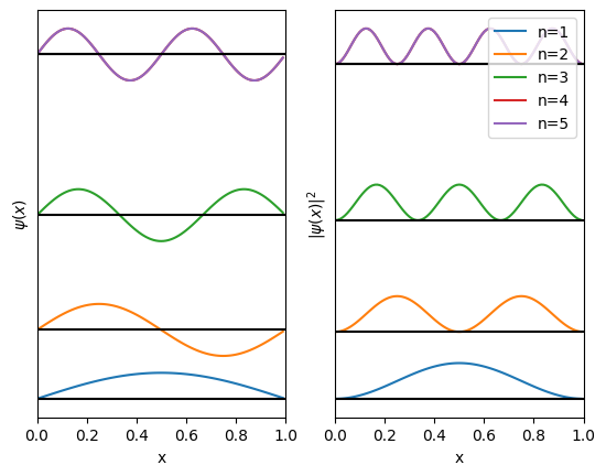
We make the following observations:

• the spacing between energy levels increases with \(n\)

• the wave function oscillates inside the box and is zero outside of the box. As \(n\) increases, the oscillations become more rapid.

• for states with \(n > 1\), the wave function passes through zero \(n-1\) times. These points where the wave function passes through zero are called “nodes.” There is zero probability of finding the particle at a node (i.e., \(|\psi(x)|^2=0\) at the node).

• there is a kink in the wave function at the left- and right-hand edges of the box, so the wave function does not have a continuous first derivative over all space. Recall that the requirement that the wave function be smooth is lifted when the potential is not finite.

Where are we most likely to find the particle? For any \(n\), we are most likely to find the particle where \(|\psi(x)|^2\) is at a maximum. To find such a point, we first locate the stationary points by setting the first derivative of the probability density equal to zero

\[\begin{align} \frac{d}{dx}|\psi(x)|^2 = 0 \end{align}\]

and solving for \(x\). We can verify that the stationary point is a maximum by checking the sign on the second derivative of the probability density. If

\[\begin{align} \frac{d^2}{dx^2} |\psi(x)|^2 < 0 \end{align}\]

the stationary point is a maximum. For the PIB problem, all maxima in \(|\psi(x)|^2\) have the same value (meaning we’re equally likely to find the particle at any of the maxima). For other problems, this might not be the case; there could be local maxima.

How does the quantum mechanical probability density relate to the classical one? For a classical particle in a box, we would be equally likely to find the particle anywhere in the box (with probability \(1/L\)), as visualized here:

L = 1.0
hbar = 1.0
m = 1.0

x = np.arange(0, L, 0.01)

wfn_1 = np.sqrt(2.0 / L) * np.sin(1 * np.pi * x / L)
wfn_2 = np.sqrt(2.0 / L) * np.sin(2 * np.pi * x / L)

figure = plt.plot()

plt.xlim(0, 1)
plt.yticks(ticks=[])
plt.ylabel(r'$|\psi(x)|^2$')
plt.xlabel('x')
plt.plot(x, wfn_1**2, label = 'n=1')
plt.plot(x, wfn_2**2, label = 'n=2')
plt.axhline(y=1.0, color='black', label = 'classical probability')

plt.legend(loc='upper right')
plt.show()

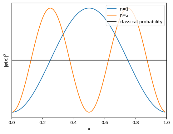
Clearly, the quantum and classical probability distributions differ, which brings us to an impoartant question. Should quantum mechanics recover classical results in any limit? The anser is yes. The Bohr Correspondence Principle states that, in the limit of large quantum numbers, quantum mechanicals will recover classical results. Let us consider the quantum mechanical description of a classical particle, which would have very large \(m\) and \(L\). Given the form of the energy:

\[\begin{align} E_n = \frac{\hbar^2 n^2 \pi^2}{2 m L^2} \end{align}\]

we can conclude that the spacings between energy levels is tiny because \(m\) and \(L\) are large. As a consequence any non-zero kinetic energy will put the particle in an extremely high-energy state. Let us inspect the probability density for a high-energy state, as compared to the low-energy states and the classical limit.

L = 1.0
hbar = 1.0
m = 1.0

x = np.arange(0, L, 0.001)

wfn_1 = np.sqrt(2.0 / L) * np.sin(1 * np.pi * x / L)
wfn_2 = np.sqrt(2.0 / L) * np.sin(2 * np.pi * x / L)
wfn_100 = np.sqrt(2.0 / L) * np.sin(100 * np.pi * x / L)

figure = plt.plot()

plt.xlim(0, 1)
plt.yticks(ticks=[])
plt.ylabel(r'$|\psi(x)|^2$')
plt.xlabel('x')
plt.plot(x, wfn_1**2, label = 'n=1')
plt.plot(x, wfn_2**2, label = 'n=2')
plt.plot(x, wfn_100**2, label = 'n=100')
plt.axhline(y=1.0, color='black', label = 'classical probability')

plt.legend(loc='upper right')
plt.show()

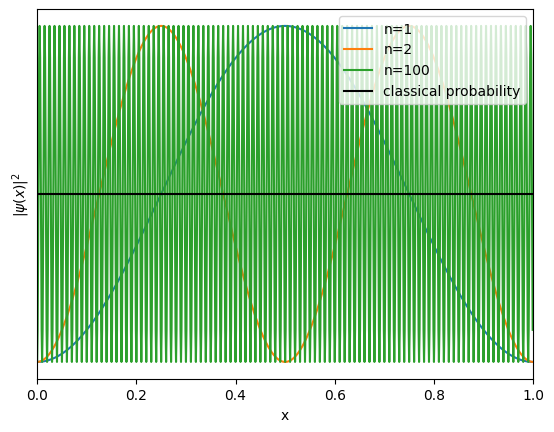
At first glance, it seems like the classical and large-\(n\) limits still yield different probability distributions, until we think about the resoultion of any actual measurement of position. For sufficiently high \(n\), the oscillations in \(|\psi_n(x)|^2\) will be sufficiently rapid that it will be impossible to resolve the difference between a maximum and a minimum in the distribution, and the classical distribution (the average of these) is what is detected.

Practice

Question 2: Show that particle-in-a-box wave functions for different states, \(n_i\) and \(n_j\) are orthogonal.

Answer 2

We have $\(\begin{align} \psi_{n_i}(x) = \left ( \frac{2}{L} \right )^{1/2} \text{sin}\left(\frac{n_i \pi x}{L}\right) \end{align}\)\( when \)0 \le x \le L\(, and \)\psi_{n_i}(x) = 0\( otherwise. The overlap of \)\psi_{n_i}(x)\( and \)\psi_{n_j}(x)\( is \)\( \begin{align} \langle \psi_{n_i} | \psi_{n_j} \rangle &= \int_{-\infty}^{0} |0|^2 dx + \frac{2}{L} \int_0^L \text{sin}\left(\frac{n_i \pi x}{L} \right )\text{sin}\left(\frac{n_j \pi x}{L} \right ) dx + \int_L^\infty |0|^2 dx \\ &= \frac{2}{L} \int_0^L \text{sin}\left(\frac{n_i \pi x}{L} \right )\text{sin}\left(\frac{n_j \pi x}{L} \right ) dx \end{align}\)\( Using the trigonometric identity \)\(\begin{align} \text{sin}(n_i x) \text{sin}(n_j x) = \frac{1}{2} \text{cos}\left[(n_i - n_j) x\right] - \frac{1}{2} \text{cos}\left[(n_i + n_j) x\right] \end{align}\)\( This overlap becomes \)\( \begin{align} \langle \psi_{n_i} | \psi_{n_j} \rangle &= \frac{1}{L} \int_0^L \left ( \text{cos}\left[\frac{(n_i - n_j) \pi x}{L} \right] - \text{cos}\left[\frac{(n_i + n_j) \pi x}{L} \right] \right ) dx \\ &= \left . \frac{1}{L} \left ( \frac{1}{n_i-n_j}\text{sin}\left[\frac{(n_i - n_j) \pi x}{L} \right] - \frac{1}{n_i+n_j}\text{sin}\left[\frac{(n_i + n_j) \pi x}{L} \right] \right ) \right |_0^L \\ &= 0 \end{align}\)\( The limit at \)x=L\( is zero because \)n_i\pm n_j$ are both integers.

Before moving on, it is worth reiterating that the application of boundary conditions placed restrictions on the form of the wave function, which then led to the quantization of the energy. Essentially, only certain wave functions satisfy the boundary conditions (i.e., are well behaved), and, thus only certain energies are observed. We can supplement these mathematical arguments for the quantization of the energy with the following, more physical arguments.

Recall that all PIB wave functions look like standing waves. If a particle is represented as a wave, then only certain wave lengths will lead to waves that do not interfere destructively with themselves. For a standing wave, the wave length should be a half-integer multiple of the box length, i.e.,

\[ \begin{align} \frac{n \lambda}{2} = L \end{align}\]

where \(n = 1, 2, 3,\) etc. Now, recall the de Broglie wave length for a microscopic particle, which is related to the linear momentum, \(p\), for that particle

\[\begin{align} \lambda = \frac{h}{p} \end{align}\]

If we insert the de Broglie wave length into the standing wave length expression and solve for the momentum, we obtain

\[\begin{align} p = \frac{n h}{2 L} \end{align}\]

For the particle-in-a-box problem, the energy is purely kinetic because the potential is zero inside the box and the wave function is zero outside the box. Combining the classical expression for the kinetic energy and the expression above for the momentum yields

\[\begin{align} E = \frac{p^2}{2m} = \frac{n^2 h^2}{8 mL^2} \end{align}\]

which is the same result obtained from solving the Schrödinger equation and applying boundary conditions! In this case, simple physical arguments starting from the wave-like nature of microscopic particles leads to the same result as solving the Schrödinger equation directly.

Deeper Dive on the modeling of conjugated dyes

As discussed in this interview, there are some exciting applications that can be opened up by desigining chromophores that absorb or emit Short Wave Infrared radiation (SWIR). It turns out to be difficult to design organic chromophores that absorb and emit in this region with high efficiency.

We discussed the particle in a box model as being particularly useful for thinking about electronic transitions in cyanine dyes. While this model would also suggest that we can abritrarily red-shift such dyes by increasing the number of conjugated pi units, and that while we do, the cyanine dyes would become better absorbers and emitters.
As we discuss in the episode, this is not actually true for reasons that are very interesting and somewhat complicated (please listen to find out more!).

That said, the scaling relationships suggested by the particle in a box model are interesting in their own right, and useful in some limited contexts, so we try to illustrate them here!

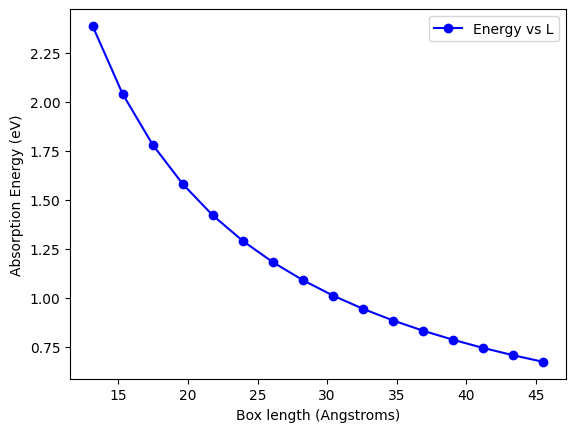
🔬 Particle in a Box: Length and Energy Scaling in a Cyanine Dye

Let’s explore how the HOMO–LUMO gap scales in a conjugated dye using a 1D particle-in-a-box model.

The energy levels are given by:

\[ E_n = \frac{\hbar^2 \pi^2 n^2}{2mL^2} \]

The length of the “box” is approximated by:

\[ L = a(K + 1) + b \]

Where:

• \( a = 2.49 \) Å

• \( b = 5.69 \) Å

• \( L \) is the number of –CH=CH– units

We assume:

\[ n_{\text{HOMO}} = K + 3 \]

---

🧮 Step 1: Unit Conversion — Angstroms to Meters

Let’s start by converting the length of the box from Ångströms to meters.

Prompt:
For \( K = 5 \), compute the box length \( L \) in Ångströms and convert it to meters.

Click to reveal the solution

First, calculate \( L \):

\[ L = 2.49(5 + 1) + 5.69 = 2.49 \times 6 + 5.69 = 20.63\ \text{Å} \]

Now convert to meters:

\[ 1\ \text{Å} = 1 \times 10^{-10}\ \text{m} \]

So:

\[ L = 20.63 \times 10^{-10} = 2.063 \times 10^{-9}\ \text{m} \]

---

⚡ Step 2: Energy in Joules

Use the particle-in-a-box equation to compute the HOMO–LUMO gap in Joules.

Prompt:
For \(K = 5 \), we have \( n_{\text{HOMO}} = 8 \) and \( n_{\text{LUMO}} = 9 \).
Compute the energy difference \( \Delta E = E_9 - E_8 \) in Joules.

Click to reveal the solution

Let’s plug into:

\[ E_n = \frac{\hbar^2 \pi^2 n^2}{2mL^2} \]

Constants:

• \( \hbar = 1.055 \times 10^{-34} \ \text{J·s} \)

• \( m = 9.109 \times 10^{-31} \ \text{kg} \)

• \( L = 2.063 \times 10^{-9} \ \text{m} \)

Compute:

\[ \Delta E = \frac{\hbar^2 \pi^2}{2mL^2} (n_{\text{LUMO}}^2 - n_{\text{HOMO}}^2) = C \cdot (9^2 - 8^2) \]

where

\[ C = \frac{(1.055 \times 10^{-34})^2 \cdot \pi^2}{2 \cdot 9.11 \times 10^{-31} \cdot (2.063 \times 10^{-9})^2} \approx 1.4156 \times 10^{-20}\ \text{J} \]

Then:

\[ \Delta E = C \cdot (81 - 64) = C \cdot 17 \approx 2.406 \times 10^{-19} \ \text{J} \]

---

⚙️ Step 3: Convert to Electronvolts (eV)

Prompt:
Convert your answer from Joules to electronvolts.
Use:
\( 1\ \text{eV} = 1.602 \times 10^{-19} \ \text{J} \)

Click to reveal the solution

Convert:

\[ \Delta E = \frac{2.406 \times 10^{-19}\ \text{J}}{1.602 \times 10^{-19}\ \text{J/eV}} \approx 1.502\ \text{eV} \]

---

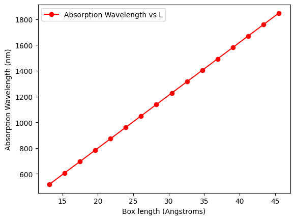
🌈 Step 4: Convert to Wavelength (nm)

Prompt:
Use the relation \( E = \frac{hc}{\lambda} \) to find the wavelength (in nm) corresponding to this energy.

Use:

• \( h = 6.626 \times 10^{-34} \ \text{J·s} \)

• \( c = 3.00 \times 10^8 \ \text{m/s} \)

Click to reveal the solution

Rearrange:

\[ \lambda = \frac{hc}{\Delta E} = \frac{6.626 \times 10^{-34} \cdot 3.00 \times 10^8}{2.406 \times 10^{-19}} \approx 8.26 \times 10^{-7}\ \text{m} \]

Convert to nm:

\[ \lambda \approx 826\ \text{nm} \]

This corresponds to the short infrared region.

---

✅ Summary

For \( K = 5 \), we find:

• \( L = 2.063 \times 10^{-9}\ \text{m} \)

• \( \Delta E \approx 2.406 \times 10^{-19}\ \text{J} \approx 1.502\ \text{eV} \)

• \( \lambda \approx 826\ \text{nm} \)

This illustrates how quantum size effects can explain optical properties of molecules!

The next code block will illustrate these scaling relationships.

from scipy import constants
# create an array for k, where k is the number of -CH=CH- units.
# basically each value of k defines a new cyanine dye with a longer "box length"
k = np.linspace(2,15,16)

# a constant in SI units related to the average -CH=CH- unit length
a = 2.49e-10
# b constant in SI units related to the length of the terminal moities in 
# the cyanine dyes
b = 5.69e-10

# create an array of L values, where L is the length of the box,
# for each distinct dye defined by the k array
L = a * (k + 1) + b

# create an array of quantum numbers associated with the HOMOs of each dye
n_homo = k + 3

# create an array of quantum numbers associated with the LUMOs of each dye
n_lumo = k + 4

# need reduced Planck's constant and the mass of the electron in SI units as well
hbar = constants.hbar
m = constants.m_e
h = constants.h
c = constants.c

# conversion from SI units of energy (Joules) to electron volts
ev_to_joules = 1.602e-19


# compute the energies of each HOMO in SI units
E_homo = hbar ** 2 * np.pi ** 2 * n_homo ** 2 / (2 * m * L ** 2)
# compte the energies of each LUMO in SI units
E_lumo = hbar ** 2 * np.pi ** 2 * n_lumo ** 2 / (2 * m * L ** 2)

# energy gaps in eV
E_gap = (E_lumo - E_homo)
E_gap_eV = E_gap / ev_to_joules


# absorption wavelength in nm 
lambda_abs = ( h * c ) / E_gap * 1e9

# plot of the absorption energy of each dye vs it's "box length"
plt.plot(L*1e10, E_gap_eV, 'bo-', label='Energy vs L')
plt.xlabel("Box length (Angstroms)")
plt.ylabel("Absorption Energy (eV)")
plt.legend()
plt.show()

# plot of the absorption wavelength of each dye vs it's "box length"
plt.plot(L*1e10, lambda_abs, 'ro-', label='Absorption Wavelength vs L')
plt.xlabel("Box length (Angstroms)")
plt.ylabel("Absorption Wavelength (nm)")
plt.legend()
plt.show()

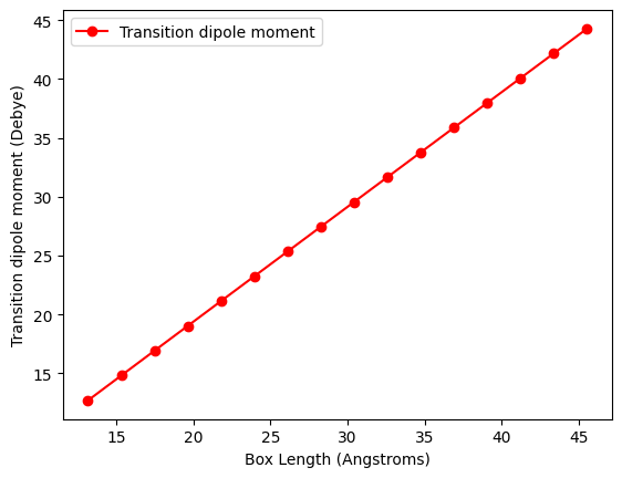
The second trend of interest is the scaling of the transition dipole moment with the size of the cyanine system, which we can again estimate from the particle in a box system. Here, we want to compute the transition dipole moment between the particle in a box energy eigenfunctions that are reasonable models for the HOMO and LUMO orbitals: $\( \mu_{n_i\rightarrow n_f} = \int_0^L \psi_{n_f}(x) \: \hat{\mu} \: \psi_{n_i}(x) dx. \)\( Here, the particle in a box energy eigenfunctions have the form \)\( \psi_n(x) = \sqrt{\frac{2}{L}} \: {\rm sin}\left( \frac{n \pi x}{L} \right), \)\( and the transition dipole operator has the form \)\( \hat{\mu} = -e x \)\( where \)e\( is the electron charge and \)x\( is displacement or position operator along the \)x$ axis. The full expression for the transition dipole moment integrals can be found on page 5 of the supporting information of this paper.

Given that the quantum numbers for the HOMO-LUMO transitions always differ by one, the relevant HOMO-LUMO transition dipole moments from the particle in a box model take on a fairly simple form as follows: $\( \mu_{i\rightarrow f} = 2eL \left( \frac{1}{( n_f + n_i )^2 \pi^2 } - \frac{1}{\pi^2} \right). \)\( From this, we can see that the transition dipole moment approaches a value of \)\frac{-2eL}{\pi^2}\( in the limit of large \)k\( (which is also the limit of large \)L\(); thus from this particle in a box model, we would expect the transition dipole momento to scale linearly with the length of the cyanine dye system. We see from the plot below, this is the case! Note in the podcast, we could not remember how it scaled and speculated it scaled as the square root of \)L\(, so we were being too conservative by a factor of \)L^{1/2}$!

# charge of the electron
ec = constants.elementary_charge
# compute the transition dipole moment in SI units for the above values of L
mu = 2 * ec * L * (1/((n_lumo + n_homo)**2 * np.pi**2) - 1/np.pi**2)

# conversion from SI units of dipole to Debye
cm_to_debye =  1 / 3.33564e-30 

# plot of the transition dipole moment of the particle in a box
# HOMO-LUMO transitions vs "box length"
plt.plot(L*1e10, np.abs(mu*cm_to_debye), 'ro-', label='Transition dipole moment')
plt.xlabel("Box Length (Angstroms)")
plt.ylabel("Transition dipole moment (Debye)")
plt.legend()
plt.show()

Three-Dimensional Particle-in-a-Box

Now, consider the three-dimensional generalization of the PIB problem. In the three-dimensional PIB problem, a particle of mass, \(m\), is confined to a three-dimensional region of space by an infinite potential barrier. In this problem, the potential has the form

\[\begin{split} \begin{align} V(x,y,z) = 0 \text{, } \text{if } &0 \le x \le a \\ \text{and } &0 \le y \le b \\ \text{and } &0 \le z \le c \end{align}\end{split}\]

and

\[ \begin{align} V(x, y, z) = \infty \text{, otherwise} \end{align}\]

We showed above that the wave function is zero in regions of space where the potential is infinite, so we only need to solve the Schrödinger equation for the wave function inside the box. We have

\[\begin{align} \hat{H}\psi(x, y, z) = E\psi(x, y, z) \end{align}\]

with

\[\begin{align} \hat{H} = -\frac{\hbar^2}{2m} \nabla^2 = -\frac{\hbar^2}{2m} \left ( \frac{\partial^2}{\partial x^2} + \frac{\partial^2}{\partial y^2} + \frac{\partial^2}{\partial z^2} \right ) \end{align}\]

Note that the Hamiltonian is additively separable in \(x\), \(y\), and \(z\). This structure means that we can apply the separation of variables technique, as was done in the time-independent Schrödinger equation in the previous notebook. The wave function will be a product of wave functions that depend, separately on each variable, i.e.,

\[ \begin{align} \psi(x, y, z) = f(x) g(y) h(z) \end{align}\]

Insert this result into the Schrödinger equation to obtain

\[ \begin{align} -\frac{\hbar^2}{2m} \left [ f^{\prime\prime}(x) g(y) h(z) + f(x) g^{\prime\prime}(y) h(z) + f(x) g(y) h^{\prime\prime}(z) \right ] = E f(x) g(y) h(z) \end{align}\]

Left-multiplying both sides of the equation by \(\frac{1}{f(x) g(y) h(z)}\) yields

\[\begin{align} -\frac{\hbar^2}{2m} \frac{1}{f(x)} f^{\prime\prime}(x)-\frac{\hbar^2}{2m} \frac{1}{g(x)} g^{\prime\prime}(y)-\frac{\hbar^2}{2m} \frac{1}{h(x)} h^{\prime\prime}(z) = E \end{align}\]

or

\[\begin{align} E_x + E_y + E_z = E \end{align}\]

with

\[ \begin{align} E_x = -\frac{\hbar^2}{2m} \frac{1}{f(x)} f^{\prime\prime}(x) \end{align}\]

etc. Now, it is easy to see that, for

\[ \begin{align} E_x = E - E_y + E_z \end{align}\]

the left-hand side depends only on the variable \(x\), while the right-hand side depends on \(y\) and \(z\) and is independent of \(x\). So, if \(x\) is varied and \(y\) and \(z\) are held constant, then the right-hand side of this equation will not change. Hence, \(E_x\), \(E_y\), and \(E_z\) must all be constants.

The functions \(f(x)\), \(g(y)\), and \(h(z)\) can be determined by solving separate one-dimensional problems of the form

\[\begin{split}\begin{align} \frac{d^2}{dx^2} f(x) &= -\frac{2 m E_x}{\hbar^2} f(x) \\ \frac{d^2}{dy^2} g(y) &= -\frac{2 m E_y}{\hbar^2} g(y) \\ \frac{d^2}{dz^2} h(z) &= -\frac{2 m E_z}{\hbar^2} h(z) \end{align}\end{split}\]

While look like the equation for the one-dimensional PIB problem, with similar boundary conditions. Hence,

\[\begin{split} \begin{align} f(x) &= \left ( \frac{2}{a} \right )^{1/2} \text{sin}\left ( \frac{n_x \pi x}{a} \right ) \\ g(y) &= \left ( \frac{2}{b} \right )^{1/2} \text{sin}\left ( \frac{n_y \pi y}{b} \right ) \\ h(z) &= \left ( \frac{2}{c} \right )^{1/2} \text{sin}\left ( \frac{n_z \pi z}{c} \right ) \end{align}\end{split}\]

where \(n_x\), \(n_y\), and \(n_z\) are all positive integers, and

\[ \begin{align} \psi(x, y, z) = \left ( \frac{8}{abc} \right )^{1/2} \text{sin}\left ( \frac{n_x \pi x}{a} \right ) \text{sin}\left ( \frac{n_y \pi y}{b} \right )\text{sin}\left ( \frac{n_z \pi z}{c} \right ) \end{align}\]

For the energy, we have

\[\begin{split}\begin{align} E_x &= \frac{n_x^2 h^2}{8ma^2} \\ E_y &= \frac{n_y^2 h^2}{8mb^2} \\ E_z &= \frac{n_z^2 h^2}{8mc^2} \end{align}\end{split}\]

and

\[ \begin{align} E = \frac{h^2}{8m}\left ( \frac{n_x^2}{a^2} + \frac{n_y^2}{b^2} + \frac{n_z^2}{c^2} \right ) \end{align}\]

The ground state (the lowest-energy state) will have \(n_x = n_y = n_z = 1.\)

Degenerate Energy Levels

Suppose that the box to which the particle is confined is a cube, with \(a = b = c.\) The energy would be

\[ \begin{align} E = \frac{h^2}{8ma^2}\left ( n_x^2 + n_y^2 + n_z^2 \right ) \end{align}\]

Now, states with different quantum numbers could be degenerate. The table below provides values of \(n_x^2 + n_y^2 + n_z^2,\) which is proportional to the energy, for the lowest 11 states.

\(n_x\)	\(n_y\)	\(n_z\)	\(n_x^2 + n_y^2 + n_z^2\)	\(g\)
1	1	1	3	1
2	1	1	6	3
1	2	1	6	3
1	1	2	6	3
2	2	1	9	3
2	1	2	9	3
1	2	2	9	3
3	1	1	11	3
1	3	1	11	3
1	1	3	11	3
2	2	2	12	1

We can see that the ground state is non-degenerate, but the first, second, and third excited states are all triply degenerate.

It is easy to visualize why some states are degenerate. Consider an electron of mass, \(m = m_e\), confined to a two-dimensional box with sides, \(a = b = 1a_0\). Following a procedure similar to that given above, the wave function and energy levels for this state are

\[ \begin{align} \psi(x, y) = \frac{2}{a} \text{sin}\left ( \frac{n_x \pi x}{a}\right )\text{sin}\left ( \frac{n_y \pi y}{a}\right ) \end{align}\]

and

\[ \begin{align} E = \frac{h^2}{8ma^2} \left ( n_x^2 + n_y^2 \right ) \end{align}\]

Let us visualize the wave functions for the lowest-energy excited states, which are degenerate and characterized by \(n_x = 1,\) \(n_y = 2\) and \(n_x = 2,\) \(n_y = 1.\).

x, y = np.mgrid[0:1:101j, 0:1:101j]

psi_12 = 2.0 * np.sin(1 * np.pi * x) * np.sin(2 * np.pi * y)
psi_21 = 2.0 * np.sin(2 * np.pi * x) * np.sin(1 * np.pi * y)

fig, (ax1, ax2) = plt.subplots(1, 2)

#ax1.plot(psi_12, 'title = '

ax1.set_xticks(ticks=[])
ax2.set_xticks(ticks=[])
ax1.set_yticks(ticks=[])
ax2.set_yticks(ticks=[])

ax1.imshow(psi_12, label = r'$n_x = 1$, $n_y = 2$')
ax2.imshow(psi_21, label = r'$n_x = 2$, $n_y = 1$')

<matplotlib.image.AxesImage at 0x10504b1c0>

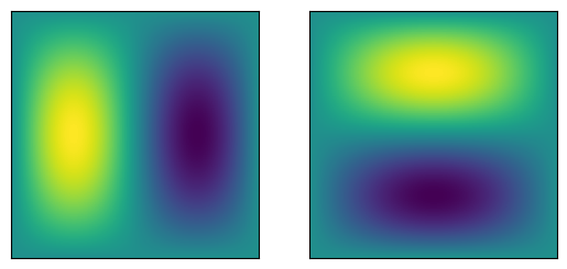
We can see that these wave functions look identical, except for their spatial orientation, so it is not surprising that the states have the same energy.

The Free Particle, Revisited

Now that we have some practice applying boundary conditions, let’s revisit the free particle problem. Recall that the Schrödinger equation for a particle of mass, \(m\), moving in the \(x\)-direction and subject to no external forces has the form

\[\begin{split}\begin{align} -\frac{\hbar^2}{2m} \frac{d^2}{dx^2} \psi(x) &= E \psi(x) \\ \frac{d^2}{dx^2} \psi(x) &= -\frac{2mE}{\hbar^2} \psi(x) \\ \frac{d^2}{dx^2} \psi(x) &= -k^2 \psi(x) \end{align}\end{split}\]

where \(k = +\left (\frac{2mE}{\hbar^2}\right)^{1/2}\). We already found that this equation has a general solution

\[ \begin{align} \psi(x) = A e^{ikx} + B e^{-ikx} \end{align}\]

Can we apply any boundary conditions? We do not know much about the form of the wave function as \(x \to \pm \infty\), aside from the fact that it does not go to zero, i.e.,

\[ \begin{align} \lim_{x\to\pm\infty} \psi(x) \neq 0 \end{align}\]

As such, there is a non-zero probability that the particle could be found anywhere in \(x\), even at \(x \to \pm \infty.\) Such a state is called an “unbound” state, as opposed to a “bound” state in which the particle is localized in some region of space. For a bound state,

\[ \begin{align} \lim_{x\to\pm\infty} \psi(x) = 0 \end{align}\]

While the free-particle wave function does not vanish as \(x\to\pm\infty\), we should still expect that it is finite in this limit, i.e.,

\[ \begin{align} \lim_{x\to\pm\infty} |\psi(x)| < \infty \end{align}\]

This is the only boundary condition for the free particle problem: the wave function must be finite everywhere. Does this condition have any interesting consequences?

Let us assume that \(E < 0\) and see what happens to the wave function

\[\begin{split}\begin{align} \psi(x) &= A e^{i[2mE / \hbar^2]^{1/2} x} + B e^{-i[2mE / \hbar^2]^{1/2} x} \\ &= A e^{i[-2m|E| / \hbar^2]^{1/2} x} + B e^{-i[-2m|E| / \hbar^2]^{1/2} x} \\ &= A e^{-[2m|E| / \hbar^2]^{1/2} x} + B e^{[2m|E| / \hbar^2]^{1/2} x} \end{align}\end{split}\]

Now, consider the following limits

\[ \begin{align} \lim_{x \to \infty} \psi(x) = A e^{-\infty} + B e^{\infty} = B e^{\infty} = \infty \end{align}\]

and

\[ \begin{align} \lim_{x \to -\infty} \psi(x) = A e^{\infty} + B e^{-\infty} = A e^{\infty} = \infty \end{align}\]

So, \(E<0\) leads to \(\psi(\pm\infty) = \infty\), which violates our only boundary condition. As such, \(E\) must be a non-negative number. This result makes sense, physically. The energy of a free particle is purely kinetic. Classically, the kinetic energy, \(T\), is

\[ \begin{align} T = \frac{p^2}{2m} \end{align}\]

Having \(T < 0\) would imply that the momentum is imaginary! This result is clearly nonsense and is rejected as non-physical.

Practice

Question 3: Prove that the expectation value of the kinetic energy operator in the \(x\) direction is non-negative.

Answer 3

We would like to show:

\[\langle \hat{T}_x \rangle = \frac{\langle \psi | \hat{T}_x | \psi \rangle}{\langle \psi | \psi \rangle} \ge 0\]

To simplify things, let us assume that \(\psi\) is normalized, i.e., \(\langle \psi | \psi \rangle = 1\), so we have:

\[\langle \hat{T}_x \rangle = \langle \psi | \hat{T}_x | \psi \rangle\]

\[= \int_{-\infty}^{\infty} \psi(x)^* \frac{\hat{p}_x^2}{2m} \psi(x) \, dx\]

\[= \frac{1}{2m} \int_{-\infty}^{\infty} \psi(x)^* \hat{p}_x \hat{p}_x \psi(x) \, dx\]

\[= \frac{1}{2m} \int_{-\infty}^{\infty} \psi(x)^* \hat{p}_x f(x) \, dx\]

where we have introduced a function \(f(x) = \hat{p}_x \psi(x)\).

Now, because \(\hat{p}_x\) is Hermitian, the last line can be re-expressed as:

\[\langle \hat{T}_x \rangle = \frac{1}{2m} \left( \int_{-\infty}^{\infty} f(x)^* \hat{p}_x \psi(x) \, dx \right)^*\]

\[= \frac{1}{2m} \left( \int_{-\infty}^{\infty} f(x)^* f(x) \, dx \right)^*\]

\[= \frac{1}{2m} \int_{-\infty}^{\infty} f(x)^* f(x) \, dx\]

\[= \frac{1}{2m} \int_{-\infty}^{\infty} |f(x)|^2 \, dx\]

The square modulus of any function is a non-negative function,
the integral of a non-negative function over all space is non-negative,
and the mass \(m\) is also non-negative.

Therefore:

\[\langle \hat{T}_x \rangle \ge 0\]

Finite Square Well Potential

The PIB model is a crude but useful model for understanding the energy states of a confined quantum mechanical particle. Some aspects of the model are unphysical, though, nameley that, no matter how much kinetic energy the particle has, it can never overcome the infinite potential energy barrier required to escape the box. A slightly more physically sensible model is the finite square well potential model, where the particle is confined by a finite potential of height \(V_0\). In this model, in prinicple, the particle could have sufficiently high energy to allow it to escape the box. In the analysis below, though, we will assume that the energy of this particle, \(E\), is less than \(V_0\).

Graphically, the potential has the form:

Image(url = "https://raw.githubusercontent.com/deprincelab/deprincelab.github.io/main/tutorials/jupyter_notebooks/translation/square_well_potential.png")

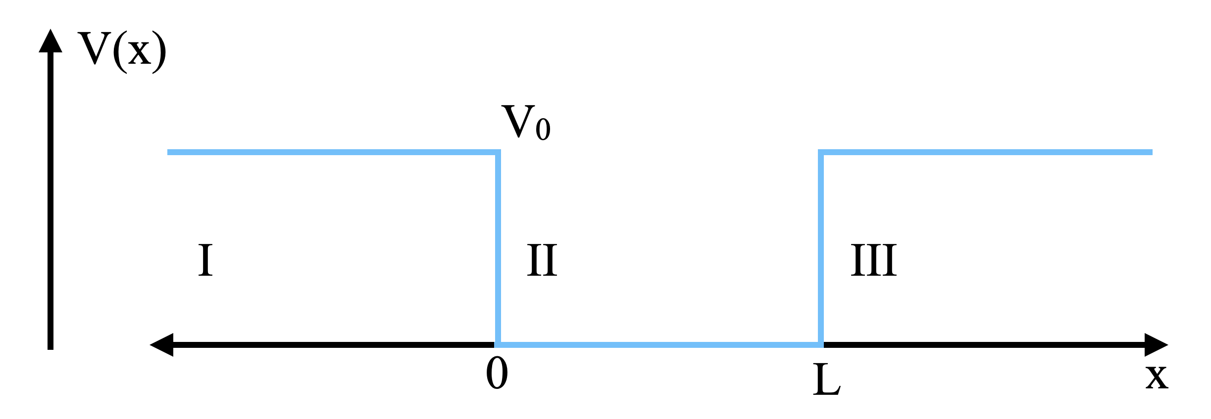
Mathematically, we define this potential in a piecewise way as

Region I (\(x < 0\)):

\[\begin{align} V(x) = V_0 \end{align}\]

Region II (\(0 \le x \le L\)):

\[\begin{align} V(x) = 0 \end{align}\]

Region III (\(x > L\)):

\[\begin{align} V(x) = V_0 \end{align}\]

Wavefunctions

As for the PIB problem, the TISE for the finite square well potential problem should be solved in a piecewise way, i.e., for each region of space. We have

Region I (\(x < 0\)):

\[\begin{align} \left ( \frac{-\hbar^2}{2m}\frac{d^2}{dx^2} + V_0 \right ) \psi_I(x) = E \psi_I(x) \end{align}\]

which has solutions of the form

\[\begin{align} \psi_I(x) = C~e^{\alpha x} + D~e^{-\alpha x} \end{align}\]

Region II (\(0 \le x \le L\)):

\[\begin{align} \frac{-\hbar^2}{2m}\frac{d^2}{dx^2} \psi_{II}(x) = E \psi_{II}(x) \end{align}\]

which has solutions of the form

\[\begin{align} \psi_{II}(x) = A~{\rm cos}(\beta x) + B~{\rm sin}(\beta x) \end{align}\]

and

Region III (\(x > l\)):

\[ \begin{align} \left (\frac{-\hbar^2}{2m}\frac{d^2}{dx^2} + V_0 \right ) \psi_{III}(x) = E \psi_{III}(x) \end{align}\]

which has solutions of the form

\[\begin{align} \psi_{III}(x) = F~e^{\alpha x} + G~e^{-\alpha x} \end{align}\]

Above, \(\alpha\) and \(\beta\) are real numbers, defined by

\[\begin{align} \alpha = ( 2 m [V_0 - E] / \hbar^2)^{1/2} \end{align}\]

\[\begin{align} \beta = (2 m E / \hbar^2)^{1/2} \end{align}\]

Note that the solutions in regions I and III involve real-valued exponential functions, as opposed to complex exponential functions.

Boundary Conditions

If we consider that the wave function should be finite in the limit that \(x\) tends to \(\pm \infty\), then we immediately find that two of the unknown coefficients must be zero. First, consider the limit

\[ \begin{align} \lim_{x\to-\infty} \psi_I(x) = Ce^{-\alpha\infty} + D e^{\alpha\infty} = D e^{\infty} \end{align}\]

Hence, \(D = 0\) is required to prevent the wave function from blowing up as \(x\to -\infty.\) Similarly, the limit

\[ \begin{align} \lim_{x\to+\infty} \psi_{III}(x) = Fe^{\alpha\infty} + G e^{-\alpha\infty} = F e^{\infty} \end{align}\]

implies that \(F\) must vanish as well. So, we have

\[\begin{split}\begin{align} \psi_{I}(x) &= C e^{\alpha x} \\ \psi_{III}(x) &= G e^{-\alpha x} \end{align}\end{split}\]

which already tells us something interesting about the probability density in regions I and III. First, there is a non-zero probability of finding the particle outside of the box, despite having \(E < V_0\). A region of space where the external potential is greater than the energy of the particle is called a classically forbidden region. It is forbidden for a classical particle to enter such a region of space, because doing so would imply that the momentum of the particle is imaginary. Classically, we would have

\[\begin{split}\begin{align} E &= T_x + V(x) \\ E - V(x) &= T_x \\ &= \frac{p_x^2}{2m} < 0\text{ if } E < V(x) \end{align}\end{split}\]

The penetration of a particle into such a classically forbidden region is called tunneling. The second interesting observation we can make is that \(|\psi(x)|^2\) will decay exponentially in these classically forbidden regions with \(E < V_0.\)

We can determine the remaining unknown coefficients through the application of additional boundary conditions:

1. The wavefunction should be continuous between regions I and II (at \(x=0\)):

   \[\begin{align} \psi_I(x=0) = \psi_{II}(x=0) \end{align}\]
   \[\begin{align} C e^{0} = A \text{cos}(0) + B\text{sin}(0) \end{align}\]
   \[\begin{align} C = A \end{align}\]

2. The derivative of the wavefunction should be continuous between regions I and II (at \(x=0\)):

   \[\begin{align} \left . \psi_I(x)^\prime \right |_{x=0} = \left . \psi_{II}(x)^\prime \right |_{x=0} \end{align}\]
   \[\begin{align} \left .C \alpha e^{\alpha x} \right |_{x=0} = \left . \left [ -\beta A \text{sin}(\beta x) + \beta B \text{cos}(\beta x) \right ] \right |_{x=0} \end{align}\]
   \[\begin{align} C \alpha e^{0} = -\beta A \text{sin}(0) + \beta B \text{cos}(0) \end{align}\]

   Inserting \(C = A\) and solving for \(B\), we have

   \[\begin{align} B = \frac{\alpha}{\beta} A \end{align}\]

   or

   \[\begin{align} B = [(V_0 - E)^{1/2} / (E)^{1/2}] A \end{align}\]

3. The wavefunction should be continuous between regions II and III (at \(x=L):\)

   \[\begin{align} \psi_{II}(x=L) = \psi_{III}(x=L) \end{align}\]
   \[\begin{align} A\text{cos}(\beta L) + \frac{\alpha}{\beta} A \text{sin}(\beta L) = G e^{-\alpha L} \end{align}\]
   \[\begin{align} G = A ~[ {\rm cos}(\beta L) + \alpha~ / \beta ~{\rm sin}(\beta L) ] ~e^{\alpha L} \end{align}\]

4. The derivative of the wavefunction should be continuous between regions II and III (at \(x=L).\) Omitting the algebra, this condition leads us to a trancendental equation for the energy:

   \[\begin{align} {\rm tan}[(2mE/\hbar^2)^{1/2} L] = 2 (V_0-E)(E)^{1/2}/(2 E-V_0) \end{align}\]

Lastly, the coefficent A can be determined by normalization.

Procedure for visualizing the allowable wavefunctions

In order to determine the allowable energies and corresponding wavefunctions for the particle in a finite square well potential, we will follow the following steps:

1. We should specify parameters \(m\), \(L\), and \(V_0\) that define our problem.

2. We should plot the trancendental equation for the energy to (a) determine how many bound states we have and (b) to obtain reasonable guesses for these energies.

3. We should numerically solve the trancendental equation using some functionality in the scipy package.

4. Once we have the allowable energies, we can evaluate the corresponding wavefunction parameters defined above.

5. Given the wave function parameters, we can visualize the wavefunction or its square modulus.

# set some parameters (in atomic units, where hbar = 1)
m = 1.0 # mass of particle
L = 1.0 # length of box (from 0 to L)
V0 = 10.0

dE = 0.01
E = np.arange(0.0, V0, dE)
#lhs = []
#rhs = []
#for i in range(len(E)):
#    lhs.append(np.tan(np.sqrt(2 * m * E[i]) * L))
#    rhs.append(2 * np.sqrt(V0-E[i]) * np.sqrt(E[i]) / (2 * E[i] - V0))
lhs = np.tan(np.sqrt(2 * m * E) * L)
rhs = 2 * np.sqrt(V0-E) * np.sqrt(E) / (2 * E - V0)

plt.figure()
plt.plot(E, lhs, marker='.', linestyle='', label = 'LHS')
plt.plot(E, rhs, marker='.', linestyle='', label = 'RHS')
plt.ylim(-10, 10)
plt.legend()
plt.show()

/var/folders/dq/61z8k56n7r3gtgfrmv5bxdxh0000gp/T/ipykernel_65410/4185230906.py:9: RuntimeWarning: divide by zero encountered in divide
  rhs = 2 * np.sqrt(V0-E) * np.sqrt(E) / (2 * E - V0)

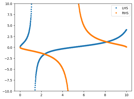
From above, we can see that there are two allowable energies (points at which the blue and orange curves cross, not counting the divergence in the blue curve). These energies look like they are roughly 2.5 and 8.0 (atomic units). We now need to numerically solve the trancendental equation. We’re going to use the function:

optimize.fsolve

from the scipy package for this purpose. We will have to pass some objective function \(f(E) = 0\) for which this function will find the optimal \(E\) value(s).

def allowable_energies(E, *data):
    """
    function defining allowable energies:

    tan[sqrt(2mE) L] - 2sqrt(V-E)sqrt(E)/(2E-V0)

    :param E: the energy
    :return value: the function value
    """
    m, V0, L = data

    return np.tan(np.sqrt(2 * m * E) * L) - 2 * np.sqrt(V0-E) * np.sqrt(E) / (2 * E - V0)

Now, we’re ready to solve for the allowable energies.

# solve for the allowable energy, with some reasonable initial guess
from scipy import optimize

E = optimize.fsolve(func = allowable_energies, x0 = [2.5, 8], args = (m, V0, L))

print('the allowable energies are', E)

the allowable energies are [2.29499075 8.13714776]

# let's plot the wave functions
alpha = np.sqrt( 2.0 * m * (V0 - E))
beta = np.sqrt( 2.0 * m * E)

A = 1 # we'll normalize, but start with A = 1
C = A
B = np.sqrt(V0 - E) / np.sqrt(E) * A
G = A * ( np.cos(beta * L) + alpha / beta * np.sin(beta * L) ) * np.exp(alpha * L)

Given the allowable energies, we can calculate the corresponding wavefunction parameters. Since all of the parameters can be expressed in terms of \(A\), we start with the choice \(A = 1\), but we’ll rescale all of the coefficients such that the wavefunction is normalized.

# define the wave function

dx = 0.01

x = np.arange(-10 * L , 11 * L, dx) 

psi = []
psi2 = []
for myx in x:
    if myx < 0:
        mypsi = C * np.exp(alpha * myx)
        psi.append(mypsi)
        psi2.append(np.abs(mypsi)**2) # in case psi is complex valued
    elif myx < L:
        mypsi = A * np.cos(beta * myx) + B * np.sin(beta * myx)
        psi.append(mypsi)
        psi2.append(np.abs(mypsi)**2)
    else :
        mypsi = G * np.exp(-alpha * myx)
        psi.append(mypsi)
        psi2.append(np.abs(mypsi)**2)

psi = np.array(psi)
psi2 = np.array(psi2)

# normalize the wave function ... 
# it is possible to do this analytically, but let's do it numerically

# N = (1 / int(|psi|^2) )^1/2

for state in range (0, len(alpha)):
    N = np.sqrt(1.0 / np.trapz(psi2[:, state], x = x))
    psi[:, state] *= N
    psi2[:, state] *= N*N

/var/folders/dq/61z8k56n7r3gtgfrmv5bxdxh0000gp/T/ipykernel_65410/337456428.py:7: DeprecationWarning: `trapz` is deprecated. Use `trapezoid` instead, or one of the numerical integration functions in `scipy.integrate`.
  N = np.sqrt(1.0 / np.trapz(psi2[:, state], x = x))

# plot normalized wave functions overlaid over the potential

Vx = []
for xval in x:
    if xval < 0.0:
        Vx.append(V0)
    elif xval < L:
        Vx.append(0.0)
    else:
        Vx.append(V0)

Vx = np.array(Vx)

plt.figure()
plt.plot(x, psi)
plt.plot(x, Vx * 0.1)
plt.xlim(-1, 2)
plt.show()

Practice

Now, you should re-run this part of the notebook with different values for the mass (\(m\)), the width of the well (\(L\)), and the height of the potential outside of the well (\(V_0\)). Ask yourself the following questions:

---

Question 4: Does increasing \(V_0\) increase or decrease the number of bound states?

Answer 4

As \(V_0\) is increased, the well should be able to support a larger number of bound states.

---

Question 5: Does increasing \(L\) increase or decrease the number of bound states?

Answer 5

As \(L\) is increased, the well should be able to support a larger number of bound states.

We can rationalize this result by thinking about the form of the energy for the infinite square well potential model (the particle in a box):

\[E_n = \frac{h^2 n^2}{8mL^2}\]

As \(L\) increases, the spacing between energy levels decreases. Hence, for the finite square well potential model, it is reasonable to expect that a similar trend will occur, resulting in a larger number of states with \(E < V_0\).

---

Question 6: Does increasing \(m\) increase or decrease the number of bound states?

Answer 6

As \(m\) is increased, the well should be able to support a larger number of bound states.

Again, we can rationalize this result by thinking about the form of the energy for the infinite square well potential model (the particle in a box):

\[E_n = \frac{h^2 n^2}{8mL^2}\]

As \(m\) increases, the spacing between energy levels decreases. Hence, for the finite square well potential model, it is reasonable to expect that a similar trend will occur, resulting in a larger number of states with \(E < V_0\).

---

Question 7: For a given \(m\), \(L\), and \(V_0\), which bound states have the highest / lowest tunneling probability (the probability of finding the particle outside of the well)? Can you rationalize this result?

Answer 7

The highest-energy bound states should have the largest tunneling probability.
The lowest-energy bound states should have the lowest tunneling probability.

We can rationalize this result by considering the form of the wave function in region III:

\[\psi_{III}(x) = G e^{-\alpha x}\]

Recall that:

\[\alpha = \sqrt{\frac{2 m [V_0 - E]}{\hbar^2}}\]

The quantity \(V_0 - E\) is related to how rapidly the wave function decays with increasing \(x\) in this region of space.
As \(E\) increases, \(V_0 - E\) decreases, which implies that the wave function will decay more slowly in this region.

---

Question 8: Can the number of bound states ever be zero, for certain combinations of \(m\), \(L\), and \(V_0\)?

Answer 8

No, the minimum number of bound states is one, no matter what values we have for \(m\), \(L\), and \(V_0\).

This ananlysis has assumed that the potential barrier height, \(V_0\), is greater than the energy for the particle, \(E\). What if \(E > V_0\)? In this case, the particle should be able to overcome the potential barrier to “escape” the box. Let us inspect the general form of the wave function in region I given above, (before the application of any boundary conditions). We had

\[ \begin{align} \psi_I(x) = A e^{\alpha x} + B^{-\alpha x} \end{align}\]

with

\[ \begin{align} \alpha = \left ( \frac{2m}{\hbar^2} \right )^{1/2} \left ( V_0 - E \right )^{1/2} \end{align}\]

which must be imaginary, since \(V_0 - E < 0\)! A similar analysis holds for the wave function in region III. Hence the wave function looks like sums of complex exponential functions in all regions of space, much like the wave function for a free particle. Moreover

\[\begin{align} \lim_{x\to-\infty} \psi_I(x) \neq 0 \end{align}\]

and

\[ \begin{align} \lim_{x\to+\infty} \psi_{III}(x) \neq 0 \end{align}\]

which implies that there is a non-zero probability of finding the particle anywhere in \(x\). Hence, the states with \(E > V_0\) are unbound states. Like in the free-particle problem, the energy for these unbound states is continuous (not quantized).

Tunneling Through a Barrier

The finite square well potential model demonstrated that a quantum particle can penetrate into a classically forbidden region. We can extend this concept by considering a situation where a particle of mass, \(m\), and energy, \(E\), encounters a potential energy barrier of height, \(V_0 > E\), and width, \(L\). Graphically, we have the following situation

Image(url = "https://raw.githubusercontent.com/deprincelab/deprincelab.github.io/main/tutorials/jupyter_notebooks/translation/tunneling_through_barrier.png")

where we have assumed that the particle encounters the barrier from the left (from the \(-x\) direction). Classical mechanics would predict that the particle would be reflected off of the potential barrier, given that the barrier height exceeds the energy. On the other hand, quantum mechanics suggests that it is possible for the particle to tunnel into the barrier, and, possibly, be transmitted through to the other side.

What is the probability, \(T\), that the particle will be transmitted through the barrier? To answer this question, let us first define the wave function in each region. As in the previous examples, the wave function is defined in a piecewise manner, by solving the Schrödinger equation in each region. We have

Region I (\(x < 0\)):

\[\begin{align} V(x) = 0 \end{align}\]

\[\begin{align} \frac{-\hbar^2}{2m}\frac{d^2}{dx^2} \psi_I(x) = E \psi_I(x) \end{align}\]

which has solutions of the form

\[\begin{align} \psi_I(x) = A~e^{ikx} + B~e^{-ikx} \end{align}\]

Region II (\(0 \le x \le L\)):

\[\begin{align} V(x) = V_0 \end{align}\]

\[\begin{align} (\frac{-\hbar^2}{2m}\frac{d^2}{dx^2} + V_0) \psi_{II}(x) = E \psi_{II}(x) \end{align}\]

which has solutions of the form

\[\begin{align} \psi_{II}(x) = C~e^{\lambda x} + D~e^{-\lambda x} \end{align}\]

and

Region III (\(x > L\)):

\[\begin{align} V(x) = 0 \end{align}\]

\[\begin{align} \frac{-\hbar^2}{2m}\frac{d^2}{dx^2} \psi_{III}(x) = E \psi_{III}(x) \end{align}\]

which has solutions of the form

\[\begin{align} \psi_{III}(x) = F~e^{i k x} + G~e^{-i k x} \end{align}\]

Above, \(k\) and \(\lambda\) are real numbers, defined by

\[\begin{align} k = (2 m E / \hbar^2)^{1/2} \end{align}\]

\[\begin{align} \lambda = ( 2 m [V_0 - E] / \hbar^2)^{1/2} \end{align}\]

Similar to the finite square well potential problem, the solutions in regions I and III (where \(V(x) = 0\)) involve complex exponential functions, while the solution in region II (where \(V(x) = V_0 > E\)) involves real-valued exponential functions.

How can we define the transmission probability? First, note that the wave functions in regions I and III look like free partile wave functions. Such wave functions are a superposition of momentum eigenfunctions, and the probability amplitudes are related to the probability that the particle will be found moving to the right / left in a particular region of space. Specifically,

• \(|A|^2\) is proportional to the probability that the particle is traveling to the right in region I

• \(|B|^2\) is proportional to the probability that the particle is traveling to the left in region I

• \(|F|^2\) is proportional to the probability that the particle is traveling to the right in region III

• \(|G|^2\) is proportional to the probability that the particle is traveling to the left in region III

The tunneling probability should be probability that the particle is traveling to the right in region III, normalized by the probability that the particle encountered the barrier in region I, or

\[ \begin{align} T = \frac{|F|^2}{|A|^2} \end{align}\]

Similarly, we could define a reflection probability, \(R\), as the probability that the particle is moving to the left in region I, normalized by the probability that the particle encountered the barrier in region I, or

\[ \begin{align} R = \frac{|B|^2}{|A|^2} \end{align}\]

In order to determine \(T\), we must apply boundary conditions to determine the unknown coefficients, \(A\), \(B\), \(C\), \(D\), \(F\), and \(G\). We have four boundary conditions:

1. The wave function should be continuous between regions I and II: \(\psi_I(x=0) = \psi_{II}(x=0)\)

2. The derivative of the wave function should be continuous between regions I and II: \(\left . \psi^\prime_I(x) \right |_{x=0} = \left . \psi_{II}^\prime(x) \right |_{x = 0}\)

3. The wave function should be continuous between regions II and III: \(\psi_{II}(x=L) = \psi_{III}(x=L)\)

4. The derivative of the wave function should be continuous between regions II and III: \(\left . \psi^\prime_{II}(x) \right |_{x=L} = \left . \psi_{III}^\prime(x) \right |_{x = L}\)

At first glance, it seems like we have more unknown coefficients than equations, but this will not be an issue. First, we can eliminate one of the unknowns on physical grounds. Consider the coffficient, \(G\). The value \(|G|^2\) should represent the probability that the particle is moving to the left in region III. However, because (i) the particle encountered the barrier from the left and (ii) the potential in region III is zero for all \(x > L\), we can conclude that the particle should never be found moving to the left in region III. Therefore, we set \(G = 0\). Second, note that we do not need to know \(A\) and \(F\) absolutely. Determining \(T\) only requires knowledge of their ratio. Hence, we really only have four unknown quantities:

\[ \begin{align} \frac{|F|^2}{|A|^2}\text{, }B\text{, }C\text{, }D \end{align}\]

Boundary condition 1:

Enforcing continuity of the wave function at the boundary between regions I and II \([ \psi_I(x=0) = \psi_{II}(x=0)]\) leads to

\[\begin{split}\begin{align} A e^0 + B e^0 &= C e^0 + D e ^0 \\ A + B &= C + D \end{align}\end{split}\]

Enforcing the smoothness of the wave function at the boundary between regions I and II \([ \left . \psi^\prime_I(x) \right |_{x=0} = \left . \psi_{II}^\prime(x) \right |_{x = 0} ]\) leads to

\[\begin{split}\begin{align} ik A e^0 - ik B e^0 &= \lambda c e^0 - \lambda D e^0 \\ ik (A - B) &= \lambda (C - D) \\ A - B &= -\frac{i\lambda}{k} (C - D) \\ \end{align}\end{split}\]

Adding the results of the application of these boundary conditions eliminates \(B\) and leads to

\[ \begin{align} 2 A = C\left ( 1 - \frac{i\lambda}{k}\right ) + D \left ( 1 + \frac{i\lambda}{k}\right ) \end{align}\]

Eventually after applying the two remaining conditions and a bit of algebra, we eventually find

\[\begin{split} \begin{align} T &= \frac{|F|^2}{|A|^2} \\ &= \left [ 1 + \frac{V_0^2}{4E(V_0-E)}\text{sinh}\left ( \left [ \frac{2m(V_0-E)}{\hbar^2}\right ]^{1/2} L \right ) \right ]^{-1} \end{align}\end{split}\]

where the hyperbolic sine function is defined by

\[\begin{align} \text{sinh}(x) = \frac{e^x - e^{-x}}{2} \end{align}\]

This expression for \(T\) is a bit difficult to interpret directly, but we can learn something useful in the limits of high (\(V_0 - E \gg 1\)) and wide (\(L \gg 1\)) barriers. For the hyperbolic sine term, we have

\[\begin{split} \begin{align} \lim_{\substack{V_0 - E \gg 1\\ L \gg 1}} \text{sinh}\left ( \left [ \frac{2m(V_0-E)}{\hbar^2}\right ]^{1/2} L \right ) &= \frac{1}{2} \lim_{\substack{V_0 - E \gg 1\\ L \gg 1}} \left [ e^{[2m(V_0-E)/\hbar^2]^{1/2}L} - e^{-[2m(V_0-E)/\hbar^2]^{1/2}L} \right ] \\ &= \frac{1}{2} e^{[2m(V_0-E)/\hbar^2]^{1/2}L} \end{align}\end{split}\]

Now,

\[\begin{split} \begin{align} \lim_{\substack{V_0 - E \gg 1\\ L \gg 1}}T &= \left [ 1 + \frac{V_0^2}{8E(V_0-E)}\frac{1}{2} e^{[2m(V_0-E)/\hbar^2]^{1/2}L} \right ]^{-1} \\ &\approx \frac{8E(V_0-E)}{V_0^2}e^{-[2m(V_0-E)/\hbar^2]^{1/2}L} \end{align}\end{split}\]

This last expression is much easier to interpret. The tunneling probability, \(T\), decreases as

• \(L\) increases

• \(V_0 - E\) increases

• \(m\) increases

Hence, tunneling is most important for light particles encountering low, narrow barriers.